Probabilistic PCA

[01/04/2024] Update: Review Singular Value Decomposition (SVD).

First, let’s review PCA (Principal Component Analysis) model. PCA is a linear dimensionality reduction technique that seeks to find the directions of maximum variance in high-dimensional data. The first principal component is the direction in which the data varies the most. The second principal component is orthogonal to the first and captures the remaining variance. The third principal component is orthogonal to the first two, and so on. The principal components are the eigenvectors of the covariance matrix of the data. The eigenvalues of the covariance matrix represent the variance of the data along the corresponding eigenvectors.

Given an $N \times D$ data matrix $X = {x_1, x_2, \ldots, x_N}$, where $x_i \in \mathbb{R}^D$, PCA seeks to find a $D \times K$ matrix $W$ such that the projected data $Z = {z_1, z_2, \ldots, z_N}$, where $z_i \in \mathbb{R}^K$, maximizes the variance of the data. The projected data is given by $Z = XW$. The columns of $W$ are the principal components.

So, why we need dimensionality reduction? There are several reasons:

1. Data compression: By reducing the dimensionality of the data, we can store the data more efficiently. $K$ is usually much smaller than $D$.
2. Visualization: It is difficult to visualize high-dimensional data. By reducing the dimensionality of the data, we can visualize the data in a lower-dimensional space.
3. Noise reduction: By reducing the dimensionality of the data, we can remove noise from the data. The noise is usually in the directions of low variance. How PCA could minimize the noise? The noise is in the directions of low variance, and PCA seeks to find the directions of maximum variance. Therefore, the noise is projected onto the directions of low variance and is removed.
4. Learning faster: By reducing the dimensionality of the data, we can reduce the computational cost of learning algorithms. The learning algorithms are usually faster in lower-dimensional spaces.
5. Avoid overfitting: We can also avoid overfitting by reducing the dimensionality of the data. Overfitting occurs when the model is too complex and captures the noise in the data.

On the other hand, we don’t want to lose too much information of $X$ when we project it to $Z$, preserving the useful information and discarding the rest. And there are many ways to quantify the information loss.

Before diving into the PCA and PPCA, let’s review some basic concepts in linear algebra.

Eigenvalues and eigenvectors

Given a square matrix $A \in \mathbb{R}^{D \times D}$, a non-zero vector $v \in \mathbb{R}^D$ is an eigenvector of $A$ if $Av = \lambda v$, where $\lambda \in \mathbb{R}$ is the eigenvalue corresponding to the eigenvector $v$. The eigenvectors of $A$ are orthogonal if $v_i^Tv_j = 0$ for $i \neq j$. The eigenvectors of $A$ form a basis for $\mathbb{R}^D$ if $A$ has $D$ linearly independent eigenvectors.

We can write the eigendecomposition of $A$ as $A = Q\Lambda Q^{-1}$, where $Q$ is a matrix whose columns are the eigenvectors of $A$, and $\Lambda$ is a diagonal matrix whose diagonal elements are the eigenvalues of $A$. If $A$ is symmetric, then $A = Q\Lambda Q^T$.

Real quick we note here how to compute the eigenvectors and eigenvalues of a matrix $A$:

1. Compute the characteristic polynomial of $A$: $\text{det}(A - \lambda I) = 0$, where $I$ is the identity matrix.
2. Solve the characteristic equation to find the eigenvalues $\lambda$.
3. For each eigenvalue $\lambda$, solve the equation $(A - \lambda I)v = 0$ to find the eigenvectors $v$.
4. Normalize the eigenvectors to have unit length.
5. The eigenvectors are orthogonal if $A$ is symmetric.
6. The eigenvectors form a basis for $\mathbb{R}^D$ if $A$ has $D$ linearly independent eigenvectors. The eigenvectors are the principal components of the data.

Singular value decomposition (SVD)

Given a matrix $X \in \mathbb{R}^{N \times D}$, the singular value decomposition (SVD) of $X$ is given by $X = U\Sigma V^T$, where $U \in \mathbb{R}^{N \times N}$, $\Sigma \in \mathbb{R}^{N \times D}$, and $V \in \mathbb{R}^{D \times D}$. The columns of $U$ are the left singular vectors of $X$, the columns of $V$ are the right singular vectors of $X$, and the diagonal elements of $\Sigma$ are the singular values of $X$. The singular values are non-negative and are sorted in descending order $\sigma_1 \geq \sigma_2 \geq \ldots \geq \sigma_D \geq 0$. I would recommend you to read the proof of SVD.

The SVD of $X$ can be used to compute the eigendecomposition of the covariance matrix of $X$. The covariance matrix of $X$ is given by $\Sigma = \frac{1}{N}X^TX$. The eigenvectors of $\Sigma$ are the right singular vectors of $X$, and the eigenvalues of $\Sigma$ are the squares of the singular values of $X$.

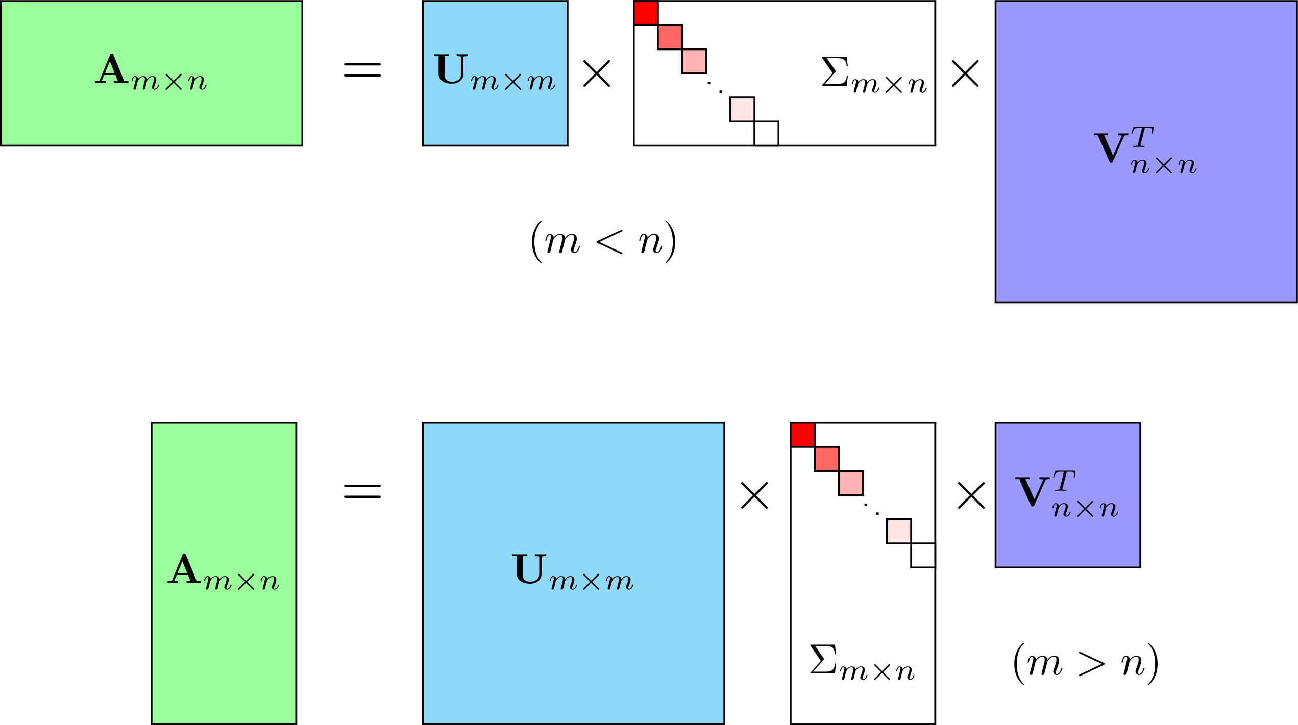Figure 1: Visualization of Singular Value Decomposition (SVD) for different shapes of matrices. The top equation shows the SVD for a matrix $A$ where the number of rows $m$ is less than the number of columns $n$. It is decomposed into $U$, $\Sigma$, and $V^T$ matrices where $U$ is an $m \times m$ matrix, $\Sigma$ is an $m \times n$ diagonal matrix, and $V^T$ is an $n \times n$ matrix. The lower equation shows the SVD for a matrix $A$ where $m$ is greater than $n$, with $U$ as an $m \times m$ matrix, $\Sigma$ as an $m \times n$ diagonal matrix, and $V^T$ as an $n \times n$ matrix.

Why called it “singular” value decomposition?

Given that $X = U\Sigma V^T$, the singular values are the square roots of the eigenvalues of $X^TX$ or $XX^T$. The singular values are singular because they are the square roots of the eigenvalues of the singular matrices $X^TX$ or $XX^T$. The singular values are the square roots of the eigenvalues of the covariance matrix of $X$.

Orthogonal & Orthonormal matrices

A matrix $Q \in \mathbb{R}^{D \times D}$ is orthogonal if $Q^TQ = I$, where $I$ is the identity matrix. The columns of an orthogonal matrix are orthonormal, i.e., $q_i^Tq_j = 0$ for $i \neq j$ and $q_i^Tq_i = 1$. The inverse of an orthogonal matrix is its transpose, i.e., $Q^{-1} = Q^T$.

In the context of PCA, the matrix $W$ is orthogonal. The columns of $W$ are the principal components of the data. The principal components are orthogonal to each other, i.e., $w_i^Tw_j = 0$ for $i \neq j$.

Principal Component Analysis (PCA)

As we mentioned earlier, PCA seeks to find a $D \times K$ matrix $W$ such that the projected data $Z = XW$ maximizes the variance of the data. The columns of $W$ are the principal components of the data. So the principal components are directions in the data that capture the most variance.

The first principal component is the direction in which the data varies the most. The second principal component is orthogonal to the first and is direction of the next highest variance. The third principal component is orthogonal to the first two and is the direction of the next highest variance, and so on. PCA takes the top $K$ principal components and projects the data onto these directions.

So we can quickly summarize it mathematically:

Given $N$ data points $X = {x_1, x_2, \ldots, x_N}$, where $x_i \in \mathbb{R}^D$, our goal is to project the data onto a $K$-dimensional subspace, where $K < D$. Let $w_1, w_2, \ldots, w_K$ be the principal components of the data. The projected data is given by $Z = XW$, where $W = [w_1, w_2, \ldots, w_K]$. The columns of $W$ are the principal components of the data. We assume that $W$ is orthogonal $W^TW = I$ and that the columns of $W$ are normalized $w_i^Tw_i = 1$.

In case $K = 1$, the first principal component is the direction in which the data varies the most. The first principal component is the eigenvector of the covariance matrix of the data that corresponds to the largest eigenvalue. We write the problem as:

\[\max_{w_1} \frac{1}{N} \sum_{i=1}^N (x_i^Tw_1)^2 \quad \text{s.t.} \quad w_1^Tw_1 = 1.\]

The solution to the above problem is the eigenvector of the covariance matrix of the data that corresponds to the largest eigenvalue. The first principal component is the direction in which the data varies the most.

In case $K > 1$, we suppose that $w_1 \in \mathbb{R}^D$ is the first principal component. Then the solution for second principal component $w_2$ is the eigenvector is:

\[\begin{aligned} \max_{w_2} \frac{1}{N} \sum_{i=1}^N (x_i^Tw_2)^2 \\ \text{s.t.} \quad w_2^Tw_2 = 1 \\ w_2^Tw_1 = 0. \end{aligned}\]

And so on for the third, fourth, and so on principal components.

We can prove this statement by using the Lagrange multiplier method. The Lagrangian is given by:

\[\mathcal{L}(w_2, \lambda) = \frac{1}{N} \sum_{i=1}^N (x_i^Tw_2)^2 - \lambda(w_2^Tw_2 - 1) - \mu w_2^Tw_1,\]

where $\lambda$ and $\mu$ are the Lagrange multipliers. We take the derivative of the Lagrangian with respect to each variable and set it to zero. We get the following equations:

\[\begin{aligned} \frac{\partial \mathcal{L}}{\partial w_2} &= \frac{2}{N} \sum_{i=1}^N x_i(x_i^Tw_2) - 2\lambda w_2 - \mu w_1 = 0 \\ \frac{\partial \mathcal{L}}{\partial \lambda} &= w_2^Tw_2 - 1 = 0 \Leftrightarrow w_2^Tw_2 = 1 \\ \frac{\partial \mathcal{L}}{\partial \mu} &= w_2^Tw_1 = 0. \end{aligned}\]

To continue, we multiply the first equation by $w_1^T$ and use the fact that $w_1^Tw_2 = 0$ to get:

\[\begin{aligned} & \frac{2}{N} \sum_{i=1}^N x_i(x_i^Tw_2) - 2\lambda w_2 - \mu w_1 &= 0 \\ &\Leftrightarrow \frac{2}{N} \sum_{i=1}^N x_i(x_i^Tw_2) - 2\lambda w_2 &= 0 \\ &\Leftrightarrow \frac{2}{N} \sum_{i=1}^N x_i(x_i^Tw_2) &= 2\lambda w_2 \\ &\Leftrightarrow \frac{1}{N} \sum_{i=1}^N x_i(x_i^Tw_2) &= \lambda w_2. \end{aligned}\]

The last equation is the eigenvector equation of the covariance matrix of the data. Therefore, the solution to the above problem is the eigenvector of the covariance matrix of the data that corresponds to the second largest eigenvalue. The second principal component is the direction in which the data varies the second most.

So on, we can find the third, fourth, and so on principal components by solving the eigenvector equation of the covariance matrix of the data.

\[\begin{aligned} \max_{w_i} \frac{1}{N} \sum_{i=1}^N (x_i^Tw_i)^2 \\ \text{s.t.} \quad w_i^Tw_i = 1 \\ w_i^Tw_j = 0 \quad \text{for} \quad i \neq j. \end{aligned}\]

The solution to the above problem is the eigenvector of the covariance matrix of the data that corresponds to the $i$-th largest eigenvalue. The $i$-th principal component is the direction in which the data varies the $i$-th most.

To resume PCA, we can summarize it as step by step:

• Step 1: Compute the mean of the data $m = \frac{1}{N} \sum_{i=1}^N x_i$.
• Step 2: Subtract the mean from the data $x_i = x_i - m$.
• Step 3: Compute the covariance matrix of the data $\Sigma = \frac{1}{N}X^TX$.
• Step 4: Compute the eigendecomposition of the covariance matrix $\Sigma = Q\Lambda Q^T$.
• Step 5: Take the top $K$ eigenvectors of the covariance matrix $W = [q_1, q_2, \ldots, q_K]$.
• Step 6: Project the data onto the principal components $Z = XW$.
• Step 7: The projected data $Z$ is the lower-dimensional representation of the data.

The PCA is a deterministic model. In the next section, we will introduce the probabilistic PCA (PPCA) model, which is a probabilistic model of PCA.

Probabilistic PCA (PPCA)

Probabilistic PCA was introduced by Tipping and Bishop (1999). PPCA is a probabilistic model of PCA. The PPCA model is a generative model that assumes that the data is generated by a linear transformation of a lower-dimensional latent variable plus Gaussian noise. The PPCA model is a latent variable model that seeks to find the latent variables of the data.

So, we can write $x_i = Wz_i + \mu + \epsilon_i$, where $x_i \in \mathbb{R}^D$ is the observed data, $z_i \in \mathbb{R}^K$ is the latent variable, $W \in \mathbb{R}^{D \times K}$ is the linear transformation matrix, $\mu \in \mathbb{R}^D$ is the mean of the data, and $\epsilon_i \sim \mathcal{N}(0, \sigma^2I)$ is the Gaussian noise. The latent variable $z_i$ is the lower-dimensional representation of the data.

\[x_i = \sum_{k=1}^K w_kz_{ik} + \mu + \epsilon_i.\]

So we assume that a Gaussian prior on low-dimensional representation $p(z_i) = \mathcal{N}(0, I)$, and the likelihood of the data given the latent variable is $p(x_i \vert z_i) = \mathcal{N}(Wz_i + \mu, \sigma^2I)$. The PPCA model is a linear Gaussian model.

\[p(x_i) = \int p(x_i|z_i)p(z_i)dz_i = \mathcal{N}(Wz_i + \mu, \sigma^2I).\]

The marginal likelihood of the data is a Gaussian distribution with mean zero and covariance matrix $WW^T + \sigma^2I$. The covariance matrix of the data is given by $WW^T + \sigma^2I$. The covariance matrix of the data is a low-rank matrix, where the rank is $K$. The rank of the covariance matrix is the number of non-zero eigenvalues of the covariance matrix.

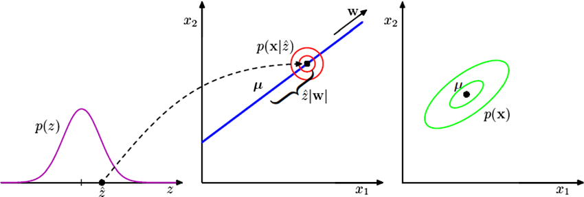Figure 2: On the left, the latent variable distribution $p(z)$ is shown. In the middle, the transformation of the latent variable into the observed space is depicted by the vector $w$, with the conditional probability $p(x|z)$ indicating variability around the transformation. On the right, the distribution of observed data $p(x)$ with its mean $\mu$ and covariance is presented.

We could do Maximum Likelihood Estimation (MLE) and Expectation-Maximization (EM) to estimate the parameters of the PPCA model.

Let note here what we got so far:

• Prior: $p(z_i) = \mathcal{N}(0, I)$
• Likelihood: $p(x_i \vert z_i) = \mathcal{N}(Wz_i + \mu, \sigma^2I)$
• Marginal likelihood: $p(x_i) = \int p(x_i \vert z_i)p(z_i)dz_i = \mathcal{N}(0, WW^T + \sigma^2I)$
• Parameters: $W$, $\mu$, $\sigma^2$
• Objective: maximize the marginal likelihood of the data

I will expand the marginal likelihood of the data $p(x_i)$:

\[\begin{aligned} p(x_i) &= \int p(x_i|z_i)p(z_i)dz_i \quad \text{Marginalize over $z_i$} \\ &= \int \mathcal{N}(x_i | Wz_i + \mu, \sigma^2I) \times \mathcal{N}(z_i | 0, I) dz_i \quad \text{// Gaussian densities} \\ &= \int (2\pi)^{-\frac{D}{2}}|\sigma^2I|^{-\frac{1}{2}}\exp\left(-\frac{1}{2}(x_i - Wz_i - \mu)^T(\sigma^2I)^{-1}(x_i - Wz_i - \mu)\right) \\ &\quad \times (2\pi)^{-\frac{K}{2}}|I|^{-\frac{1}{2}}\exp\left(-\frac{1}{2}z_i^Tz_i\right) dz_i \quad \text{// Apply density formulas} \\ &= (2\pi)^{-\frac{D}{2}}(\sigma^2)^{-\frac{D}{2}}(2\pi)^{-\frac{K}{2}} \int \exp\left(-\frac{1}{2\sigma^2}(x_i - Wz_i - \mu)^T(x_i - Wz_i - \mu)\right) \\ &\quad \times \exp\left(-\frac{1}{2}z_i^Tz_i\right) dz_i \quad \text{// Simplify using $|A| = a^n$ for $A=aI$} \\ &= (2\pi)^{-\frac{D+K}{2}}(\sigma^2)^{-\frac{D}{2}} \int \exp\left(-\frac{1}{2\sigma^2}(x_i - Wz_i - \mu)^T(x_i - Wz_i - \mu) - \frac{1}{2}z_i^Tz_i\right) dz_i \quad \text{// Combine constants} \\ \end{aligned}\]

The term inside the exponential is a quadratic form. We can expand the quadratic form and complete the square:

\[\begin{aligned} &-\frac{1}{2\sigma^2}(x_i - Wz_i - \mu)^T(x_i - Wz_i - \mu) - \frac{1}{2}z_i^Tz_i \\ &= -\frac{1}{2\sigma^2}(x_i^Tx_i - 2x_i^TWz_i + z_i^TW^TWz_i + \mu^T\mu - 2\mu^TWz_i - 2x_i^T\mu + 2z_i^TW^T\mu) - \frac{1}{2}z_i^Tz_i \quad \text{// Expand and rearrange} \\ &= -\frac{1}{2\sigma^2}(x_i - \mu)^T(x_i - \mu) -\frac{1}{2\sigma^2}z_i^TW^TWz_i + \frac{1}{\sigma^2}z_i^TW^T(x_i - \mu) - \frac{1}{2}z_i^Tz_i \quad \text{// Group terms} \\ &= -\frac{1}{2\sigma^2}(x_i - \mu)^T(x_i - \mu) + \frac{1}{\sigma^2}z_i^TW^T(x_i - \mu) -\frac{1}{2} \left( \frac{1}{\sigma^2}z_i^TW^TWz_i + z_i^Tz_i \right) \quad \text{// Factor out $\frac{1}{\sigma^2}$} \\ &= -\frac{1}{2\sigma^2}(x_i - \mu)^T(x_i - \mu) + \frac{1}{\sigma^2}z_i^TW^T(x_i - \mu) -\frac{1}{2} \left( \frac{1}{\sigma^2}z_i^TW^TWz_i + \frac{\sigma^2}{\sigma^2}z_i^Tz_i \right) \quad \text{// Adjust $z_i^Tz_i$ term for completion} \\ &= -\frac{1}{2\sigma^2}(x_i - \mu)^T(x_i - \mu) + \frac{1}{\sigma^2}z_i^TW^T(x_i - \mu) -\frac{1}{2\sigma^2}z_i^T(W^TW + \sigma^2I)z_i \quad \text{// Combine $z_i$ terms} \\ &= -\frac{1}{2\sigma^2}(x_i - \mu)^T(x_i - \mu) -\frac{1}{2\sigma^2} \left( z_i^T(W^TW + \sigma^2I)z_i - 2z_i^TW^T(x_i - \mu) \right) \quad \text{// Rearrange for completion} \end{aligned}\]

To complete the square, identify the quadratic form and linear form in the exponential. The quadratic form is $z_i^T(W^TW + \sigma^2I)z_i$ and the linear form is $2z_i^TW^T(x_i - \mu)$:

\(\begin{aligned} &-\frac{1}{2\sigma^2}(x_i - \mu)^T(x_i - \mu) -\frac{1}{2\sigma^2} \left( \underbrace{z_i^T(W^TW + \sigma^2I)z_i}_{\text{Quadratic form}} - \underbrace{2z_i^TW^T(x_i - \mu)}_{\text{Linear form}} \right) \end{aligned}\) \(\begin{aligned} &-\frac{1}{2\sigma^2}(x_i - \mu)^T(x_i - \mu) -\frac{1}{2\sigma^2} \left( z_i^T(W^TW + \sigma^2I)z_i - 2z_i^TW^T(x_i - \mu) \right) \quad \text{// Given quadratic and linear forms} \\ &= -\frac{1}{2\sigma^2}(x_i - \mu)^T(x_i - \mu) -\frac{1}{2\sigma^2} z_i^T(W^TW + \sigma^2I)z_i + \frac{1}{\sigma^2}z_i^TW^T(x_i - \mu) \quad \text{// Distribute $-\frac{1}{2\sigma^2}$} \\ &= -\frac{1}{2\sigma^2}(x_i - \mu)^T(x_i - \mu) + \frac{1}{\sigma^2}z_i^TW^T(x_i - \mu) -\frac{1}{2\sigma^2} z_i^T(W^TW + \sigma^2I)z_i \quad \text{// Rearrange terms for clarity} \\ &= -\frac{1}{2\sigma^2}(x_i - \mu)^T(x_i - \mu) + \text{[complete the square for $z_i$ terms]} \quad \text{// Indicate next step} \\ \end{aligned}\)

So to complete the square for the $z_i$ terms, we need to have expression in the form of $(z_i - M)^TC(z_i - M)$ where $C = W^TW + \sigma^2I$ and $M = C^{-1}W^T(x_i - \mu)$. Let’s incorporate these terms:

\[\begin{aligned} &= -\frac{1}{2\sigma^2}(x_i - \mu)^T(x_i - \mu) -\frac{1}{2\sigma^2} \left( z_i - (W^TW + \sigma^2I)^{-1}W^T(x_i - \mu) \right)^T(W^TW + \sigma^2I) \\ &\quad \times \left( z_i - (W^TW + \sigma^2I)^{-1}W^T(x_i - \mu) \right) + \underbrace{\frac{1}{2\sigma^2}(x_i - \mu)^TW(W^TW + \sigma^2I)^{-1}W^T(x_i - \mu)}_{\text{Constant term}} \\ \end{aligned}\]

Feww, we have completed the square. Now we pull out the constant term outside the integral:

\[\begin{aligned} p(x_i) &= (2\pi)^{-\frac{D+K}{2}}(\sigma^2)^{-\frac{D}{2}} \int \exp\left(-\frac{1}{2\sigma^2}{\color{red}(x_i - \mu)^T(x_i - \mu)} -\frac{1}{2\sigma^2} \left( {\color{orange}z_i} - {\color{green}(W^TW + \sigma^2I)^{-1}W^T(x_i - \mu)} \right)^T \right. \\ &\quad \left. {\color{blue}(W^TW + \sigma^2I)} \left( {\color{orange}z_i} - {\color{green}(W^TW + \sigma^2I)^{-1}W^T(x_i - \mu)} \right) \right) dz_i \\ &\quad + \frac{1}{2\sigma^2}{\color{purple}(x_i - \mu)^TW(W^TW + \sigma^2I)^{-1}W^T(x_i - \mu)} \\ &= (2\pi)^{-\frac{D+K}{2}}(\sigma^2)^{-\frac{D}{2}} \exp\left(\frac{1}{2\sigma^2}{\color{purple}(x_i - \mu)^TW(W^TW + \sigma^2I)^{-1}W^T(x_i - \mu)}\right) \\ &\quad \times \int \exp\left(-\frac{1}{2\sigma^2} {\color{red}(x_i - \mu)^T(x_i - \mu)} -\frac{1}{2\sigma^2} \left( {\color{orange}z_i^T(W^TW + \sigma^2I)z_i} - 2{\color{orange}z_i^T}{\color{green}W^T(x_i - \mu)} \right) \right) dz_i \\ &\quad \text{Apply the result of completing the square and integrating out $z_i$.} \end{aligned}\]

The integral is a Gaussian density. We can write the integral as a Gaussian density with mean $\mu_{z_i} = (W^TW + \sigma^2I)^{-1}W^T(x_i - \mu)$ and covariance matrix $\Sigma_{z_i} = \sigma^2(W^TW + \sigma^2I)^{-1}$. The integral is a Gaussian density with mean $\mu_{z_i}$ and covariance matrix $\Sigma_{z_i}$.

\[\begin{aligned} p(x_i) &= (2\pi)^{-\frac{D+K}{2}}(\sigma^2)^{-\frac{D}{2}} \exp\left(\frac{1}{2\sigma^2}(x_i - \mu)^TW(W^TW + \sigma^2I)^{-1}W^T(x_i - \mu)\right) \\ &\quad \times (2\pi)^{\frac{K}{2}}|\Sigma_{z_i}|^{-\frac{1}{2}}\exp\left(-\frac{1}{2}(z_i - \mu_{z_i})^T\Sigma_{z_i}^{-1}(z_i - \mu_{z_i})\right) \\ &= (2\pi)^{-\frac{D}{2}}|\sigma^2I + WW^T|^{-\frac{1}{2}}\exp\left(-\frac{1}{2}(x_i - \mu)^T(\sigma^2I + WW^T)^{-1}(x_i - \mu)\right) \quad \text{// Substitute $\mu_{z_i}$ and $\Sigma_{z_i}$} \\ \end{aligned}\]

Recall Bayes’ theorem, the posterior distribution of the latent variable given the data is given by: $p(z_i \vert x_i) = \frac{p(x_i \vert z_i)p(z_i)}{p(x_i)}$. We can write the posterior distribution of the latent variable given the data as:

\[\begin{aligned} p(z_i | x_i) &= \frac{(2\pi)^{-\frac{D}{2}}|\sigma^2I|^{-\frac{1}{2}}\exp\left(-\frac{1}{2\sigma^2}(x_i - Wz_i - \mu)^T(x_i - Wz_i - \mu)\right) \times (2\pi)^{-\frac{K}{2}}|I|^{-\frac{1}{2}}\exp\left(-\frac{1}{2}z_i^Tz_i\right)}{(2\pi)^{-\frac{D}{2}}|\sigma^2I + WW^T|^{-\frac{1}{2}}\exp\left(-\frac{1}{2}(x_i - \mu)^T(\sigma^2I + WW^T)^{-1}(x_i - \mu)\right)} \\ &= (2\pi)^{-\frac{K}{2}} \frac{|\sigma^2I|^{-\frac{1}{2}}}{|\sigma^2I + WW^T|^{-\frac{1}{2}}} \exp\left(-\frac{1}{2\sigma^2}(x_i - Wz_i - \mu)^T(x_i - Wz_i - \mu) \right. \\ &\quad \left. -\frac{1}{2}(x_i - \mu)^T(\sigma^2I + WW^T)^{-1}(x_i - \mu) -\frac{1}{2}z_i^Tz_i\right) \\ &= (2\pi)^{-\frac{K}{2}} |\sigma^2I + WW^T|^{\frac{1}{2}}|\sigma^2I|^{-\frac{1}{2}} \exp\left(-\frac{1}{2\sigma^2}(x_i - Wz_i - \mu)^T(x_i - Wz_i - \mu) -\frac{1}{2}z_i^Tz_i \right. \\ &\quad \left. + \frac{1}{2}(x_i - \mu)^T(\sigma^2I + WW^T)^{-1}(x_i - \mu)\right) \end{aligned}\]

Looking at the term inside the exponential, we can simplify it by expanding the quadratic form and rearranging the terms:

\[\begin{aligned} &-\frac{1}{2\sigma^2}(x_i - Wz_i - \mu)^T(x_i - Wz_i - \mu) -\frac{1}{2}z_i^Tz_i + \frac{1}{2}(x_i - \mu)^T(\sigma^2I + WW^T)^{-1}(x_i - \mu) \\ =& -\frac{1}{2\sigma^2}\left({\color{red}x_i^T(\sigma^2I)^{-1}x_i} - {\color{blue}2x_i^T(\sigma^2I)^{-1}Wz_i} - {\color{green}2x_i^T(\sigma^2I)^{-1}\mu} + {\color{orange}z_i^TW^T(\sigma^2I)^{-1}Wz_i} \right. \\ &\quad \left. + {\color{purple}2z_i^TW^T(\sigma^2I)^{-1}\mu} + {\color{brown}\mu^T(\sigma^2I)^{-1}\mu} \right) -\frac{1}{2}{\color{orange}z_i^Tz_i} \\ &+ \frac{1}{2} \left( {\color{red}x_i^T(\sigma^2I + WW^T)^{-1}x_i} - {\color{green}2x_i^T(\sigma^2I + WW^T)^{-1}\mu} + {\color{brown}\mu^T(\sigma^2I + WW^T)^{-1}\mu} \right) \end{aligned}\]

Further simplifying the terms, we can combine the terms with $x_i$, $z_i$, and $\mu$. We also notice that $(\sigma^2I)^{-1} = \frac{1}{\sigma^2}I$ and $(\sigma^2I + WW^T)^{-1} = \frac{1}{\sigma^2}I - \frac{1}{\sigma^2}W(W^TW + \sigma^2I)^{-1}W^T$:

\[\begin{aligned} =& -\frac{1}{2\sigma^2} \left( {\color{red}\frac{1}{\sigma^2}x_i^Tx_i} - {\color{blue}\frac{2}{\sigma^2}x_i^TWz_i} - {\color{green}\frac{2}{\sigma^2}x_i^T\mu} + {\color{orange}\frac{1}{\sigma^2}z_i^TW^TWz_i} + {\color{purple}\frac{2}{\sigma^2}z_i^TW^T\mu} + {\color{brown}\frac{1}{\sigma^2}\mu^T\mu} \right) -\frac{1}{2}{\color{orange}z_i^Tz_i} \\ &+ \frac{1}{2} \left( {\color{red}x_i^T\left(\frac{1}{\sigma^2}I - \frac{1}{\sigma^2}W(W^TW + \sigma^2I)^{-1}W^T\right)x_i} - {\color{green}2x_i^T\left(\frac{1}{\sigma^2}I - \frac{1}{\sigma^2}W(W^TW + \sigma^2I)^{-1}W^T\right)\mu} \right. \\ &\quad \left. + {\color{brown}\mu^T\left(\frac{1}{\sigma^2}I - \frac{1}{\sigma^2}W(W^TW + \sigma^2I)^{-1}W^T\right)\mu} \right) \\ =& -\frac{1}{2} \left( {\color{red}\frac{1}{\sigma^2}x_i^Tx_i} + {\color{red}x_i^T(\sigma^2I + WW^T)^{-1}x_i} - {\color{blue}2x_i^TWz_i} + {\color{orange}z_i^TW^TWz_i} - {\color{purple}2z_i^TW^T\mu} + {\color{orange}z_i^Tz_i} \right. \\ &\quad \left. - {\color{green}2x_i^T\mu} + {\color{brown}\mu^T\mu} - {\color{green}2x_i^T(\sigma^2I + WW^T)^{-1}\mu} + {\color{brown}\mu^T(\sigma^2I + WW^T)^{-1}\mu} \right) \\ \end{aligned}\]

In conclusion here, we have the conditional distribution of the latent variable given the data $p(z_i \vert x_i)$. The conditional distribution is a Gaussian density with mean $\mu_{z_i} = (W^TW + \sigma^2I)^{-1}W^T(x_i - \mu)$ and covariance matrix $\Sigma_{z_i} = \sigma^2(W^TW + \sigma^2I)^{-1}$. The conditional distribution is a Gaussian density with mean $\mu_{z_i}$ and covariance matrix $\Sigma_{z_i}$.

\[\begin{aligned} p(z_i | x_i) &= \mathcal{N}\left((W^TW + \sigma^2I)^{-1}W^T(x_i - \mu), \sigma^2(W^TW + \sigma^2I)^{-1}\right) \end{aligned}\]

Maximum Likelihood for PPCA

Computing the Maximum Likelihood for PPCA directly is challenging due to the complex nature of the likelihood function involved. The likelihood function for PPCA, as given by:

\[p(X) = \prod_{i=1}^N p(x_i) = \prod_{i=1}^N (2\pi)^{-\frac{D}{2}}|\sigma^2I + WW^T|^{-\frac{1}{2}}\exp\left(-\frac{1}{2}(x_i - \mu)^T(\sigma^2I + WW^T)^{-1}(x_i - \mu)\right),\]

Taking the log of the likelihood to simplify the product into a sum still results in a complex expression due to the determinant and the matrix inversion in the exponent. The log-likelihood involves terms like $\log \vert\sigma^2I + WW^T \vert$ and $(x_i - \mu)^T(\sigma^2I + WW^T)^{-1}(x_i - \mu)$, both of which are computationally demanding due to matrix operations.

If continue, MLE for $\mu$ should be $\hat{\mu} = \frac{1}{N}\sum_{i=1}^N x_i$. For $W$, we can use iterative methods or do eigenvalue decomposition of the covariance matrix. We could have result:

\[\begin{aligned} \hat{W} &= U_K(\Lambda_K - \sigma^2I)^{\frac{1}{2}}V^T \\ \hat{\sigma}^2 &= \frac{1}{D - K}\sum_{k=K+1}^D \lambda_k, \end{aligned}\]

where $U_K$ is the matrix of the first $K$ eigenvectors of the covariance matrix, $\Lambda_K$ is the diagonal matrix of the first $K$ eigenvalues of the covariance matrix, and $V$ is the matrix of the eigenvectors of the covariance matrix. The MLE for the latent variable $z_i$ is given by the mean of the conditional distribution $p(z_i \vert x_i)$.

Expectation-Maximization for PPCA

We will use EM to iteratively update the parameters of the PPCA model. The E-step involves computing the posterior distribution of the latent variable given the data $p(z_i \vert x_i)$. The M-step involves maximizing the expected log-likelihood of the data.

First, we write the complete data likelihood:

\[\begin{aligned} p(X, Z) &= \prod_{i=1}^N p(x_i, z_i) = \prod_{i=1}^N p(x_i | z_i)p(z_i) \\ &= \prod_{i=1}^N \mathcal{N}(Wz_i + \mu, \sigma^2I) \times \mathcal{N}(0, I) \\ &= \prod_{i=1}^N (2\pi)^{-\frac{D}{2}}|\sigma^2I|^{-\frac{1}{2}}\exp\left(-\frac{1}{2\sigma^2}(x_i - Wz_i - \mu)^T(x_i - Wz_i - \mu)\right) \\ &\quad \times (2\pi)^{-\frac{K}{2}}|I|^{-\frac{1}{2}}\exp\left(-\frac{1}{2}z_i^Tz_i\right) \end{aligned}\]

We ignore the constant terms w.r.t. $W$ and $\sigma^2$ in the log-likelihood.

The log-likelihood of the complete data is given by: \(\begin{aligned} \log p(X, Z) &= -\sum_{i=1}^N \left(\frac{D}{2}\log(\sigma^2) + \frac{1}{2\sigma^2}(x_i - Wz_i - \mu)^T(x_i - Wz_i - \mu) + \frac{K}{2}\log(2\pi) + \frac{1}{2}z_i^Tz_i\right) \\ &\quad \text{Start by expressing the log likelihood of $X$ and $Z$.} \\ &= -\sum_{i=1}^N \left(\frac{D}{2}\log(\sigma^2) + \frac{1}{2\sigma^2}\left((x_i - \mu)^T(x_i - \mu) - 2(x_i - \mu)^TWz_i + z_i^TW^TWz_i\right) + \frac{K}{2}\log(2\pi) + \frac{1}{2}z_i^Tz_i\right) \\ &\quad \text{Expand the quadratic term $(x_i - Wz_i - \mu)^T(x_i - Wz_i - \mu)$ to simplify the expression.} \\ &= -\sum_{i=1}^N \left(\frac{D}{2}\log(\sigma^2) + \frac{1}{2\sigma^2}(x_i - \mu)^T(x_i - \mu) - \frac{1}{\sigma^2}(x_i - \mu)^TWz_i + \frac{1}{2\sigma^2}z_i^TW^TWz_i + \frac{1}{2}z_i^Tz_i\right) \\ &\quad \text{Group similar terms together and separate terms involving the latent variables $z_i$.} \\ &= -\sum_{i=1}^N \left(\frac{D}{2}\log(\sigma^2) + \frac{1}{2\sigma^2}(x_i - \mu)^T(x_i - \mu)\right) + \sum_{i=1}^N\left(\frac{1}{\sigma^2}(x_i - \mu)^TWz_i\right) \\ &\quad - \sum_{i=1}^N\left(\frac{1}{2\sigma^2}z_i^TW^TWz_i + \frac{1}{2}z_i^Tz_i\right) \\ &\quad \text{Separate the log likelihood into three distinct sums to clarify the contribution of each term.} \\ &= -\sum_{i=1}^N \left(\frac{D}{2} \log \sigma^2 + \frac{1}{2\sigma^2} (x_i - \mu)^\top (x_i - \mu) - \frac{1}{\sigma^2} x_i^\top W^\top (x_i - \mu) + \frac{1}{2\sigma^2} x_i^\top W^\top W x_i + \frac12 x_i^\top x_i \right) \\ &\quad \text{Removing the latent variable $z_i$ and focusing solely on the observed data $x_i$.} \end{aligned}\)

In the E-step, we compute the expected value of $log p(X, Z)$ w.r.t. the posterior distribution of the latent variable given the data $p(z_i \vert x_i)$. The expected value of the log-likelihood is given by:

\[\begin{aligned} \mathbb{E}_{Z \vert X}[\log p(X, Z)] &= -\sum_{i=1}^N \left[\frac{D}{2} \log \sigma^2 + \frac{1}{2\sigma^2} (x_i - \mu)^\top (x_i - \mu) - \frac{1}{\sigma^2} \mathbb{E}[x_i^\top W^\top (x_i - \mu)] \right. \\ &\quad \left. + \frac{1}{2\sigma^2} \mathbb{E}[x_i^\top W^\top W x_i] + \frac12 \mathbb{E}[x_i^\top x_i] \right] \\ &= -\sum_{i=1}^N \left[\frac{D}{2} \log \sigma^2 + \frac{1}{2\sigma^2} (x_i - \mu)^\top (x_i - \mu) - \frac{1}{\sigma^2} \mathbb{E}[x_i]^\top W^\top (x_i - \mu) \right. \\ &\quad \left. + \frac{1}{2\sigma^2} \text{tr}(W^\top W \mathbb{E}[x_i x_i^\top]) + \frac12 \mathbb{E}[x_i^\top x_i] \right] \\ \end{aligned}\]

Compute the two terms $\mathbb{E}[x_i]$ and $\mathbb{E}[x_i^\top x_i]$:

\[\begin{aligned} \mathbb{E}[x_i] &= (\sigma^2I + WW^T)^{-1}W^T(x_i - \mu) \\ \end{aligned}\] \[\begin{aligned} \text{Cov}[x_i] &= \mathbb{E}[x_i^\top x_i] - \mathbb{E}[x_i]^\top\mathbb{E}[x_i] \\ & \Leftrightarrow \mathbb{E}[x_i^\top x_i] = \text{Cov}[x_i] + \mathbb{E}[x_i]^\top\mathbb{E}[x_i] \\ &\Leftrightarrow \mathbb{E}[x_i^\top x_i] = \sigma^2(\sigma^2I + WW^T) + \mathbb{E}[x_i]^\top\mathbb{E}[x_i] \end{aligned}\]

Plug in the values of $\mathbb{E}[x_i]$ and $\mathbb{E}[x_i x_i^\top]$ into the expected log-likelihood:

\[\begin{aligned} \mathbb{E}_{Z \vert X}[\log p(X, Z)] &= -\sum_{i=1}^N \left[\frac{D}{2} \log \sigma^2 + \frac{1}{2\sigma^2} (x_i - \mu)^\top (x_i - \mu) - \frac{1}{\sigma^2} \mathbb{E}[x_i]^\top W^\top (x_i - \mu) \right. \\ &\quad \left. + \frac{1}{2\sigma^2} \text{tr}(W^\top W \mathbb{E}[x_i x_i^\top]) + \frac12 \mathbb{E}[x_i^\top x_i] \right] \\ &= -\sum_{i=1}^N \left[\frac{D}{2} \log \sigma^2 + \frac{1}{2\sigma^2} (x_i - \mu)^\top (x_i - \mu) - \frac{1}{\sigma^2} \mathbb{E}[x_i]^\top W^\top (x_i - \mu) \right. \\ &\quad \left. + \frac{1}{2\sigma^2} \text{tr}(W^\top W (\sigma^2(\sigma^2I + WW^T) + \mathbb{E}[x_i]^\top\mathbb{E}[x_i])) + \frac12 (\sigma^2(\sigma^2I + WW^T) + \mathbb{E}[x_i]^\top\mathbb{E}[x_i]) \right] \\ \end{aligned}\]

In the M-step, we maximize the expected log-likelihood w.r.t. $W$ and $\sigma^2$. We take the derivative of the expected log-likelihood w.r.t. $W$ and $\sigma^2$ and set them to zero to find the optimal values of $W$ and $\sigma^2$.

\[\begin{aligned} \frac{\partial \mathbb{E}_{Z \vert X}[\log p(X, Z)]}{\partial W} &= 0 \\ \frac{\partial \mathbb{E}_{Z \vert X}[\log p(X, Z)]}{\partial \sigma^2} &= 0 \end{aligned}\]

For $W$, we have:

\[\begin{aligned} \frac{\partial \mathbb{E}_{Z | X}[\log p(X, Z)]}{\partial W} &= -\sum_{i = 1}^N \left[ -\frac{1}{\sigma^2} (x_i - \mu) \mathbb{E}[z_i]^\top + \frac{1}{\sigma^2} W \mathbb{E}[z_i z_i^\top] \right] = 0 \\ \implies W \sum_{i = 1}^N \mathbb{E}[z_i z_i^\top] &= \sum_{i = 1}^N (x_i - \mu) \mathbb{E}[z_i]^\top \\ \implies W &= \left( \sum_{i = 1}^N (x_i - \mu) \mathbb{E}[z_i]^\top \right) \left( \sum_{i = 1}^N \mathbb{E}[z_i z_i^\top] \right)^{-1} \\ \end{aligned}\]

For $\sigma^2$, we have:

\[\begin{aligned} \frac{\partial \mathbb{E}_{Z | X}[\log p(X, Z)]}{\partial \sigma^2} &= -\sum_{i = 1}^N \left[ \frac{D}{2\sigma^2} - \frac{1}{2\sigma^4} (x_i - \mu)^\top (x_i - \mu) + \frac{1}{\sigma^4} \mathbb{E}[z_i]^\top W^\top (x_i - \mu) - \frac{1}{2\sigma^4} \text{tr}(W^\top W \mathbb{E}[z_i z_i^\top]) \right] \\ &= -\frac{1}{\sigma^4} \left[ \frac{nD}{2}\sigma^2 - \frac{1}{2} \sum_{i = 1}^N (x_i - \mu)^\top (x_i - \mu) + \sum_{i = 1}^N \mathbb{E}[z_i]^\top W^\top (x_i - \mu) - \frac{1}{2} \sum_{i = 1}^N \text{tr}(W^\top W \mathbb{E}[z_i z_i^\top]) \right] \\ 0 &= \frac{nD}{2}\sigma^2 - \frac{1}{2} \sum_{i = 1}^N (x_i - \mu)^\top (x_i - \mu) + \sum_{i = 1}^N \mathbb{E}[z_i]^\top W^\top (x_i - \mu) - \frac{1}{2} \sum_{i = 1}^N \text{tr}(W^\top W \mathbb{E}[z_i z_i^\top]) \\ \sigma^2 &= \frac{1}{nD} \left[ \sum_{i = 1}^N (x_i - \mu)^\top (x_i - \mu) - 2 \sum_{i = 1}^N \mathbb{E}[z_i]^\top W^\top (x_i - \mu) + \sum_{i = 1}^N \text{tr}(W^\top W \mathbb{E}[z_i z_i^\top]) \right] \end{aligned}\]

And in this step, we have derived the M-step for the PPCA model. We have derived the update rules for the parameters $W$ and $\sigma^2$ in the PPCA model. The update rule for $W$ is given by:

\[\begin{cases} W &= \left( \sum_{i = 1}^N (x_i - \mu) \mathbb{E}[z_i]^\top \right) \left( \sum_{i = 1}^N \mathbb{E}[z_i z_i^\top] \right)^{-1} \\ \sigma^2 &= \frac{1}{nD} \left[ \sum_{i = 1}^N (x_i - \mu)^\top (x_i - \mu) - 2 \sum_{i = 1}^N \mathbb{E}[z_i]^\top W^\top (x_i - \mu) + \sum_{i = 1}^N \text{tr}(W^\top W \mathbb{E}[z_i z_i^\top]) \right] \end{cases}\]

So, we have derived the EM algorithm for the PPCA model.

As you can see, we go through many algebraic manipulations to derive the final results, with high probability of making mistakes. So, it is always a good idea to double-check the results and the derivations. If you find any mistakes, please do not hesitate to contact me. I will correct them as soon as possible.

Citation

@article{ta2023ppca,
  title={Probabilistic Principal Component Analysis},
  author={TA, Quyen Linh},
  journal={qlinhta.github.io},
  year={2023},
  url={https://qlinhta.github.io/blog/2023/PPCA/}
}

References

• Bishop, C. M. (2006). Pattern recognition and machine learning. springer.
• Tipping, M. E., & Bishop, C. M. (1999). Probabilistic principal component analysis. Journal of the Royal Statistical Society: Series B (Statistical Methodology), 61(3), 611-622.
• Roweis, S. T. (1998). EM algorithms for PCA and SPCA. Advances in neural information processing systems, 626-632.
• Ghahramani, Z., & Hinton, G. E. (1996). The EM algorithm for mixtures of factor analyzers. Technical Report CRG-TR-96-1, University of Toronto.