Latent Variable Models

Latent Variable Models (LVMs) offer a powerful framework for understanding the hidden structures within observed data. These models are especially useful in scenarios where the data generation process involves variables that are not directly observable. In this section, we delve into the foundational mathematics of LVMs, providing a step-by-step guide to their formulation and inference techniques.

Notation

Symbol	Meaning
$\mathbf{x}$	Observed data $\mathbf{x} = (x_1, x_2, \ldots, x_N), x_i \in \mathbb{R}^D$
$\mathbf{z}$	Latent variables $\mathbf{z} = (z_1, z_2, \ldots, z_N), z_i \in \mathbb{R}^K$
$\theta$	Model parameters
$p(\cdot)$	Probability density function
$q_{\phi}(\cdot)$	Variational distribution with parameters $\phi$
$\mathcal{L}(\phi, \theta; \mathbf{x})$	Evidence Lower Bound (ELBO)
$D_{KL}(\cdot)$	Kullback-Leibler (KL) divergence
$\mathbb{E}_{q}[\cdot]$	Expectation with respect to $q$
$\mathbf{z}_{\backslash i}$	Set of all variables except $z_i$
$\mathbf{z}^{(i)}$	Samples from the variational distribution corresponding to $\mathbf{x}^{(i)}$
$\mathbf{z}^{(t)}$	State of the Markov chain at iteration $t$
$\mathbf{z}^*$	Proposed state in the Metropolis-Hastings algorithm
$\alpha$	Acceptance probability in the Metropolis-Hastings algorithm
$Q(\theta, \theta^{(t)})$	Expected log-likelihood in the E-step of EM algorithm

Joint Probability Distribution

The joint probability distribution is the cornerstone of understanding how observed and latent variables are modeled together in LVMs. It encapsulates the probability of observing a particular set of data, $\mathbf{x}$, alongside a specific configuration of latent variables, $\mathbf{z}$, under a model defined by parameters $\theta$. Formally, it is expressed as:

\[p(\mathbf{x}, \mathbf{z} \vert \theta) = p(\mathbf{x} \vert \mathbf{z}, \theta) p(\mathbf{z} \vert \theta).\]

The breakdown of this formula is as follows: $p(\mathbf{x} \vert \mathbf{z}, \theta)$, the likelihood, signifies the model’s assumption about the data generation process. It quantifies the probability of observing the data $\mathbf{x}$ given a set of latent variables $\mathbf{z}$ and parameters $\theta$. This term is crucial because it directly ties the observed data with the hidden structures modeled by $\mathbf{z}$.

$p(\mathbf{z} \vert \theta)$, the prior, indicates our a priori assumptions about the distribution of the latent variables before any data observation. This distribution is guided by the model parameters $\theta$ and encapsulates our belief about the underlying structure of the data in the absence of direct observations.

This formula highlights the generative nature of LVMs, where the observed data is considered to be generated from a process involving latent variables.

Marginal Likelihood (Evidence)

The concept of marginal likelihood (or evidence) plays a pivotal role in understanding and evaluating the fit of LVMs to observed data. It is obtained by integrating out the latent variables from the joint probability distribution, thus providing a probability measure of the observed data $\mathbf{x}$ under the parameters $\theta$, without committing to specific values of $\mathbf{z}$. Mathematically, it is represented as:

\[p(\mathbf{x} | \theta) = \int p(\mathbf{x}, \mathbf{z} | \theta) d\mathbf{z} = \int p(\mathbf{x} | \mathbf{z}, \theta) p(\mathbf{z} | \theta) d\mathbf{z}.\]

This integration is key to understanding LVMs for several reasons:

• Summing over all possible latent configurations: The integral sums across all potential configurations of $\mathbf{z}$, effectively considering every way in which the latent variables could combine to generate the observed data. This is crucial for models where $\mathbf{z}$ represents hidden or unobservable factors influencing the data.
• Model evaluation: The marginal likelihood is a measure of how well the model parameters $\theta$ can explain the observed data $\mathbf{x}$. A higher marginal likelihood indicates a model that better accounts for the observed data, considering all possible underlying latent structures.
• Intractability: In many cases, this integral is intractable due to the complexity of the model or the high dimensionality of the latent space. This intractability is a significant challenge in LVMs and motivates the development of approximate inference techniques, such as Variational Inference and Markov Chain Monte Carlo (MCMC) methods, to estimate the marginal likelihood.

By integrating out the latent variables, the marginal likelihood abstracts away from the specifics of the hidden structures, focusing instead on the overall fit of the model to the data. This abstraction is both a strength, in terms of model evaluation and comparison, and a challenge, given the computational complexities involved in calculating the marginal likelihood for complex models.

Variational Inference (VI)

Variational Inference (VI) is a computational method used to approximate complex posterior distributions $p(\mathbf{z}\vert\mathbf{x}, \theta)$ with a simpler, parameterized distribution $q_{\phi}(\mathbf{z}\vert\mathbf{x})$, where $\phi$ denotes the set of variational parameters. This approximation becomes necessary when the direct computation of the posterior involves intractable integrals.

KL Divergence and ELBO

The KL divergence measures the difference between the variational approximation $q_{\phi}(\mathbf{z}\vert\mathbf{x})$ and the true posterior $p(\mathbf{z}\vert\mathbf{x}, \theta)$. It is defined as:

\[D_{KL}(q_{\phi}(\mathbf{z}|\mathbf{x}) \| p(\mathbf{z}|\mathbf{x}, \theta)) = \int q_{\phi}(\mathbf{z}|\mathbf{x}) \log \frac{q_{\phi}(\mathbf{z}|\mathbf{x})}{p(\mathbf{z}|\mathbf{x}, \theta)} d\mathbf{z}.\]

Expanding this using the definition of the true posterior via Bayes’ theorem, we get:

\[\begin{aligned} D_{KL}(q_{\phi}(\mathbf{z}|\mathbf{x}) \| p(\mathbf{z}|\mathbf{x}, \theta)) &= \int q_{\phi}(\mathbf{z}|\mathbf{x}) \left( \log q_{\phi}(\mathbf{z}|\mathbf{x}) - \log p(\mathbf{z}, \mathbf{x} | \theta) + \log p(\mathbf{x} | \theta) \right) d\mathbf{z} \\ &= \int q_{\phi}(\mathbf{z}|\mathbf{x}) \log q_{\phi}(\mathbf{z}|\mathbf{x}) d\mathbf{z} - \int q_{\phi}(\mathbf{z}|\mathbf{x}) \log p(\mathbf{z}, \mathbf{x} | \theta) d\mathbf{z} + \log p(\mathbf{x} | \theta) \int q_{\phi}(\mathbf{z}|\mathbf{x}) d\mathbf{z} \\ &= \mathbb{E}_{q}\left[\log q_{\phi}(\mathbf{z}|\mathbf{x})\right] - \mathbb{E}_{q}\left[\log p(\mathbf{x} | \mathbf{z}, \theta)\right] - \mathbb{E}_{q}\left[\log p(\mathbf{z} | \theta)\right] + \log p(\mathbf{x} | \theta). \end{aligned}\]

The Evidence Lower Bound (ELBO) can be derived by rearranging the terms in the KL divergence:

\[\begin{aligned} \log p(\mathbf{x} | \theta) - D_{KL}(q_{\phi}(\mathbf{z}|\mathbf{x}) \| p(\mathbf{z}|\mathbf{x}, \theta)) &= \mathbb{E}_{q}\left[\log p(\mathbf{x} | \mathbf{z}, \theta)\right] - D_{KL}(q_{\phi}(\mathbf{z}|\mathbf{x}) \| p(\mathbf{z} | \theta)) \\ &= \int q_{\phi}(\mathbf{z}|\mathbf{x}) \log p(\mathbf{x} | \mathbf{z}, \theta) d\mathbf{z} - \int q_{\phi}(\mathbf{z}|\mathbf{x}) \log \frac{q_{\phi}(\mathbf{z}|\mathbf{x})}{p(\mathbf{z} | \theta)} d\mathbf{z} \\ &= \mathcal{L}(\phi, \theta; \mathbf{x}). \end{aligned} \tag{*}\]

Maximizing the ELBO, $\mathcal{L}(\phi, \theta; \mathbf{x})$, is equivalent to minimizing the KL divergence between the variational distribution $q_{\phi}(\mathbf{z}\vert\mathbf{x})$ and the true posterior $p(\mathbf{z}\vert\mathbf{x}, \theta)$, thereby making the variational approximation as close as possible to the true posterior. This process involves adjusting the variational parameters $\phi$ to maximize the ELBO, which indirectly maximizes the marginal likelihood of the observed data under the model, a crucial aspect of fitting LVMs.

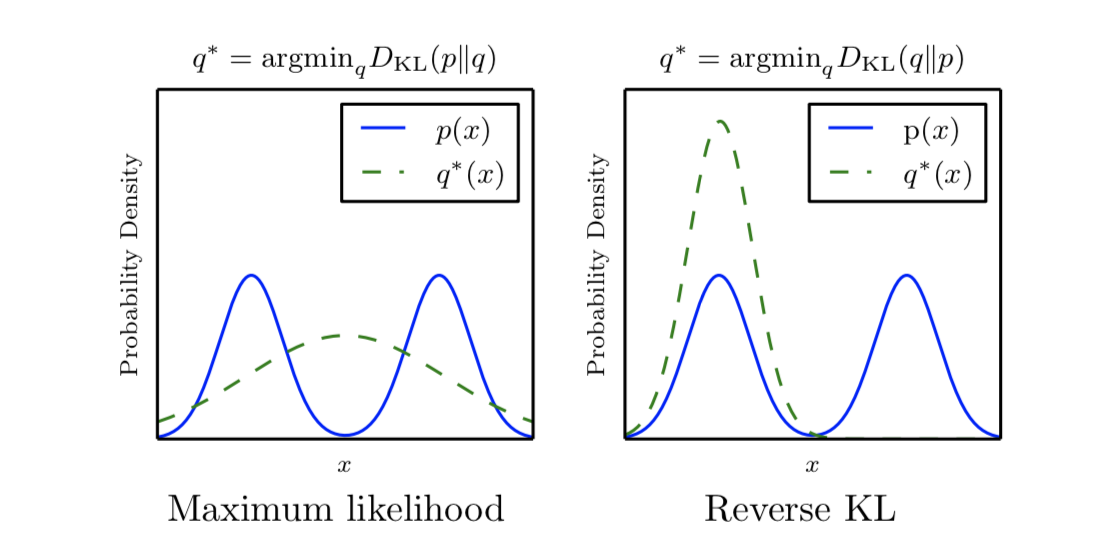Figure 1: On the left, the optimal distribution $q^*$ is obtained by minimizing the divergence from the approximate distribution to the true distribution, reflecting the maximum likelihood principle. On the right, the optimal distribution $q^*$ is found by minimizing the divergence in the opposite direction, termed the reverse divergence method. The solid blue line represents the true probability density $p(x)$, while the dashed green line represents the optimal approximate probability density $q^*(x)$.

We want to minimize the $D_{KL}(q_{\phi}(\mathbf{z}\vert\mathbf{x}) | p(\mathbf{z}\vert\mathbf{x}, \theta))$ with respect to $\phi$, which is equivalent to maximizing the ELBO $\mathcal{L}(\phi, \theta; \mathbf{x})$ with respect to $\phi$. Eric Jang’s blog post provides a detailed explanation of the derivation of the ELBO, also explain why we use $D_{KL}(q_{\phi}(\mathbf{z}\vert\mathbf{x}) | p(\mathbf{z}\vert\mathbf{x}, \theta))$ instead of $D_{KL}(p(\mathbf{z}\vert\mathbf{x}, \theta) | q_{\phi}(\mathbf{z}\vert\mathbf{x}))$.

ELBO using Jensen’s inequality

Recall: Jensen’s inequality states that for a convex function $f$, the expectation of $f(X)$ is greater than or equal to $f$ of the expectation of $X$:

\[\mathbb{E}[f(X)] \geq f(\mathbb{E}[X]).\]

Also recall that we care about $\log p(\mathbf{x} \vert \theta) = \log \int p(\mathbf{x}, \mathbf{z} \vert \theta) d\mathbf{z}$.

Using Jensen’s inequality, we can write:

\[\begin{aligned} \log p(\mathbf{x} | \theta) &= \log \mathbb{E}_{q_{\phi}(\mathbf{z}|\mathbf{x})} \left[ \frac{p(\mathbf{x}, \mathbf{z} | \theta)}{q_{\phi}(\mathbf{z}|\mathbf{x})} \right] \\ &\geq \mathbb{E}_{q_{\phi}(\mathbf{z}|\mathbf{x})} \left[ \log \frac{p(\mathbf{x}, \mathbf{z} | \theta)}{q_{\phi}(\mathbf{z}|\mathbf{x})} \right] \\ &= \mathbb{E}_{q_{\phi}(\mathbf{z}|\mathbf{x})} \left[ \log p(\mathbf{x}, \mathbf{z} | \theta) - \log q_{\phi}(\mathbf{z}|\mathbf{x}) \right] \\ &= \mathcal{L}(\phi, \theta; \mathbf{x}). \end{aligned}\]

Note that we could have the same result as in equation (*) using Jensen’s inequality, which is a more general approach to derive the ELBO.

Expectation-Maximization (EM)

The Expectation-Maximization (EM) algorithm is a fundamental tool for fitting Latent Variable Models (LVMs) when dealing with incomplete data or latent variables. It iteratively optimizes the model parameters $\theta$ by maximizing the expected log-likelihood, which involves integrating over the latent variables.

1. E-step (Expectation): Compute the expected value of the log-likelihood with respect to the posterior distribution of the latent variables, given the observed data and the current estimate of the parameters $\theta$. This step involves calculating the posterior distribution $p(\mathbf{z}\vert\mathbf{x}, \theta)$.

\[\begin{aligned} Q(\theta, \theta^{(t)}) &= \mathbb{E}_{p(\mathbf{z}|\mathbf{x}, \theta^{(t)})}[\log p(\mathbf{x}, \mathbf{z} | \theta)] \\ &= \sum_{\mathbf{z}} p(\mathbf{z}|\mathbf{x}, \theta^{(t)}) \log p(\mathbf{x}, \mathbf{z} | \theta). \end{aligned}\]

1. M-step (Maximization): Maximize the expected log-likelihood computed in the E-step with respect to the model parameters $\theta$. This step involves updating the parameters to improve the fit of the model to the observed data.

\[\theta^{(t+1)} = \arg\max_{\theta} Q(\theta, \theta^{(t)}).\]

Stochastic Variational Inference (SVI)

Stochastic Variational Inference (SVI) offers a computational framework to efficiently approximate the Evidence Lower Bound (ELBO) for large datasets by utilizing stochastic optimization techniques. The key idea is to optimize the ELBO using subsets of data (mini-batches), making the computation scalable for extensive data collections. The mathematical formulation of the SVI algorithm proceeds as follows:

1. Initialization:

   Begin with initial guesses for the variational parameters $\phi$ and the model parameters $\theta$. These parameters are crucial for defining the variational distribution $q_{\phi}(\mathbf{z}\vert\mathbf{x})$ and the model likelihood $p_{\theta}(\mathbf{x}\vert\mathbf{z})$, respectively.

2. Mini-Batch Sampling:

   At each iteration, randomly select a mini-batch of data points $\mathbf{x}^{(i)}$ from the full dataset. This selection process introduces stochasticity into the gradient estimation, aiding in scalability and convergence.

3. Gradient Estimation:

   For the selected mini-batch, estimate the gradient of the ELBO with respect to the variational parameters $\phi$, which can be expressed as:

   \[\nabla_{\phi} \mathcal{L}^{(i)}(\phi, \theta; \mathbf{x}^{(i)}) \approx \frac{N}{M} \sum_{i=1}^{M} \nabla_{\phi} \log q_{\phi}(\mathbf{z}^{(i)}|\mathbf{x}^{(i)}) [\log p_{\theta}(\mathbf{x}^{(i)}, \mathbf{z}^{(i)}) - \log q_{\phi}(\mathbf{z}^{(i)}|\mathbf{x}^{(i)})],\]

   where $N$ is the total number of data points, $M$ is the number of points in the mini-batch, and $\mathbf{z}^{(i)}$ are samples from the variational distribution corresponding to $\mathbf{x}^{(i)}$.

4. Update Variational Parameters:

   Update $\phi$ using the estimated gradient, typically with a gradient ascent step or an optimization algorithm like Adam. This step adjusts $\phi$ to improve the approximation of the posterior distribution.

5. Update Model Parameters:

   Similarly, update the model parameters $\theta$ by computing and applying the gradient of the ELBO with respect to $\theta$ for the mini-batch. This update aims to improve the model’s fit to the data.

6. Iteration:

   Repeat steps 2-5, iterating over mini-batches and sequentially updating $\phi$ and $\theta$ until the changes in the ELBO (or in the parameters) fall below a predefined threshold, indicating convergence.

SVI leverages stochastic optimization to make variational inference scalable for large datasets, addressing the computational challenges associated with evaluating the ELBO over the entire dataset. This approach enables the application of LVMs in settings where traditional variational inference methods would be prohibitively expensive, thus extending the reach of LVMs to modern, large-scale machine learning problems.

Markov Chain Monte Carlo (MCMC) Methods in LVMs

Markov Chain Monte Carlo (MCMC) methods construct a Markov chain to approximate the posterior distribution $p(\mathbf{z}\vert\mathbf{x}, \theta)$ in Latent Variable Models (LVMs), facilitating sample generation directly from the posterior.

Metropolis-Hastings Algorithm

The Metropolis-Hastings algorithm, a cornerstone of MCMC methods, generates samples by iteratively proposing and accepting or rejecting new states based on the following mathematical procedure:

1. Initialization: Begin with an initial state $\mathbf{z}_0$.

2. Proposal Step:

   Propose a new state ( \mathbf{z}^* ) from a proposal distribution ( q\left(\mathbf{z}^* \vert \mathbf{z}_t\right) ), where $\mathbf{z}_t$ is the current state:

   \[\mathbf{z}^* \sim q(\mathbf{z}^* | \mathbf{z}_t).\]

3. Acceptance Probability:

   Calculate the acceptance probability $\alpha$ for the proposed state $\mathbf{z}^*$, defined as:

   \[\alpha(\mathbf{z}_t, \mathbf{z}^*) = \min\left(1, \frac{p(\mathbf{z}^* | \mathbf{x}, \theta) q(\mathbf{z}_t | \mathbf{z}^*)}{p(\mathbf{z}_t | \mathbf{x}, \theta) q(\mathbf{z}^* | \mathbf{z}_t)}\right).\]

   This ratio balances the likelihood of moving to the new state against remaining in the current state, adjusted by the symmetry of the proposal distribution.

4. Accept/Reject Step:

   Accept the proposed state $\mathbf{z}^*$ with probability $\alpha$:

   \[\mathbf{z}_{t+1} = \begin{cases} \mathbf{z}^*, & \text{with probability } \alpha, \\ \mathbf{z}_t, & \text{with probability } 1 - \alpha. \end{cases}\]

   If the state is accepted, set $\mathbf{z}_{t+1} = \mathbf{z}^*$; otherwise, retain the current state $\mathbf{z}_t$. This acceptance step ensures that the Markov chain converges to the desired posterior distribution.

5. Iteration:

   Repeat steps 2-4, generating a sequence of samples ${\mathbf{z}_1, \mathbf{z}_2, \ldots}$ that converge to the posterior distribution.

Gibbs Sampling

Gibbs Sampling, a variant of MCMC, simplifies sampling by sequentially updating each component of $\mathbf{z}$, assuming all other components are fixed. This method is particularly effective in LVMs where conditional distributions are more tractable.

1. Initialization: Set an initial configuration $\mathbf{z}_0$.

2. Sequential Update:

   For each latent variable $z_i$, sample from its conditional distribution given all other variables and the observed data:

   \[z_i^{(t+1)} \sim p(z_i | \mathbf{z}_{\backslash i}^{(t)}, \mathbf{x}, \theta),\]

   where $\mathbf{z}_{\backslash i}^{(t)}$ represents the set of all other variables except $z_i$ at iteration $t$.

3. Iteration:

   Iterate the sequential update process, generating successive samples that collectively approximate the posterior distribution.

Comparison of VI and MCMC

MCMC methods, including Metropolis-Hastings and Gibbs Sampling, directly sample from the posterior distribution, offering an alternative to Variational Inference (VI) that optimizes a deterministic approximation. While MCMC provides a more direct approach to sampling from complex distributions, it can be computationally intensive, especially for high-dimensional models. In contrast, VI provides a computationally efficient approximation for large datasets but may introduce biases due to the choice of the variational family.

Citation

@article{ta2023latent,
  title={Latent Variable Models},
  author={TA, Quyen Linh},
  journal={qlinhta.github.io},
  year={2023},
  url={https://qlinhta.github.io/blog/2023/latent-variable-models/}
}

References

• Bishop, C. M. (2006). Pattern recognition and machine learning. Springer.
• Blei, D. M., Kucukelbir, A., & McAuliffe, J. D. (2017). Variational inference: A review for statisticians. Journal of the American Statistical Association, 112(518), 859-877.
• Gelman, A., Carlin, J. B., Stern, H. S., Dunson, D. B., Vehtari, A., & Rubin, D. B. (2013). Bayesian data analysis. CRC press.
• Murphy, K. P. (2012). Machine learning: a probabilistic perspective. MIT press.
• Neal, R. M. (2011). MCMC using Hamiltonian dynamics. Handbook of Markov Chain Monte Carlo, 2, 113-162.
• Roberts, G. O., & Rosenthal, J. S. (2004). General state space Markov chains and MCMC algorithms. Probability Surveys, 1, 20-71.
• Wainwright, M. J., & Jordan, M. I. (2008). Graphical models, exponential families, and variational inference. Foundations and Trends® in Machine Learning, 1(1-2), 1-305.