The Multi-Armed Bandit Problem

This post is still in progress. I will update it soon.

[10/04/2024] Update Upper Confidence Bound (UCB) algorithm.
[08/04/2024] Update Chernoff’s inequality proof and Diviation Inequalities.

Exploration-Exploitation Dilemma

At the heart of making choices, from the seemingly trivial to life-changing decisions, lies a tricky balancing act we all face: the exploration-exploitation dilemma. Picture this: You’re at your favorite restaurant, eyeing the menu. Do you go for that dish you know you love, or do you try something new, risking disappointment but also possibly discovering a new favorite? This everyday scenario is a perfect example of the dilemma in action. It’s about the tension between sticking with what we know works and taking a leap into the unknown, hoping it pays off. And it’s not just about choosing what to eat; exploration-exploitation dilemma plays out in the decisions we make every day, shaping everything from how we learn to how we innovate.

The bandit problem is a classic framework for studying the exploration-exploitation dilemma (Haoyu Chen, 2020; Sutton and Barto, 2018). It’s a simple yet powerful model that captures the essence of the trade-off between exploring new options and exploiting the best-known ones. The problem is named after the one-armed bandit, a type of slot machine that takes your money and gives you back a reward with some probability. The goal is to maximize the total reward you get over time by choosing which arm to pull. Each arm has an unknown reward distribution, and the challenge is to figure out which arm is the best by trying them out. The catch is that you can only pull one arm at a time, and you have to decide which arm to pull based on the rewards you’ve seen so far. This is where the exploration-exploitation dilemma comes in: do you keep pulling the arm that’s given you the most rewards so far, or do you try out a new arm in the hopes of finding an even better one?

The Bandit Problem

A bandit problem is a sequential game between a learner and an environment. The game is played $T$ times, where $T$ is the time horizon. At each time step $t \in {1, 2, \ldots, T}$, the learner chooses an action $A_t$ from a set of $\mathcal{A}$ possible actions, or arms. The goal of the learner is to maximize the total reward $\sum_{t=1}^{T} X_{A_t, t}$, where $X_{A_t, t}$ is the reward received by pulling arm $A_t$ at time $t$.

The learner’s knowledge of the environment is represented by a reward distribution for each arm. The reward distribution of arm $a \in \mathcal{A}$ is a probability distribution $P_a$ over the set of rewards $\mathcal{X}$. The learner’s goal is to learn the reward distribution of each arm and use this information to make good decisions about which arm to pull. In this post, we discuss the multi-armed bandit problem, where the learner has to choose between multiple arms, extending the classic one-armed bandit problem to a more general setting.

The history of the game up to time $t$ is denoted by:

\[\mathcal{H}_{t-1} = \{(A_1, X_{A_1, 1}), (A_2, X_{A_2, 2}), \ldots, (A_{t-1}, X_{A_{t-1}, t-1})\}\]

The learner’s decision at time $t$ is based on the history and the reward distributions $P_a$ for each arm $a \in \mathcal{A}$. The learner’s strategy is called a policy, which maps the history $\mathcal{H}_{t-1}$ to an action $A_t$.

The performance of a policy is measured by the regret, which quantifies the loss incurred by the learner due to suboptimal decisions. The regret of a policy $\pi$ is defined as the difference between the total reward obtained by the policy and the total reward that could have been obtained by pulling the best arm in hindsight:

\[\begin{align} R_T(\pi) &= \underbrace{\sum_{t=1}^{T} \max_{a \in \mathcal{A}} \mathbb{E}[X_{a, t}]}_{\text{Total reward with best arm in hindsight}} - \underbrace{\sum_{t=1}^{T} \mathbb{E}[X_{A_t, t}]}_{\text{Total reward obtained by policy $\pi$}} \\ &= \sum_{t=1}^{T} \left(\max_{a \in \mathcal{A}} \mathbb{E}[X_{a, t}] - \mathbb{E}[X_{A_t, t}]\right) \\ &= \sum_{t=1}^{T} \Delta_{A_t, t} \end{align}\]

where $\Delta_{A_t, t} = \mathbb{E}[X_{A_t, t}] - \max_{a \in \mathcal{A}} \mathbb{E}[X_{a, t}]$ is the instantaneous regret at time $t$. The regret $R_T(\pi)$ is the sum of the instantaneous regrets over the time horizon $T$.

We quickly note an example of a simple environment where the reward distributions $X_{a, t} \sim \text{Bernoulli}(\mu_a)$, where $\mu_a \in [0, 1]$ is the mean reward of arm $a$. If we knew the mean rewards $\mu_a$ for each arm, the optimal policy would be to always pull the best arm $a^* = \arg\max_{a \in \mathcal{A}} \mu_a$. The regret over $T$ time steps would be:

\[\begin{align} R_T(\pi) = \sum_{t=1}^{T} \Delta_{A_t, t} = \sum_{t=1}^{T} \left(\mu_{a^*} - \mu_{A_t}\right) \end{align}\]

The worst-case regret is defined as the maximum regret over all possible reward distributions. In the case of Bernoulli rewards, the worst-case regret is:

\[R_T(\pi) \leq \sum_{t=1}^{T} \max_{a \in \mathcal{A}} \Delta_{a, t}\]

We list the worst-case regret bounds for different types of bandit environments in the table below:

Environment	Description	Worst-Case Regret
Stationary	Reward probabilities remain constant over time.	$\mathcal{O}(\log T)$ for optimal algorithms.
Non-Stationary	Reward probabilities change over time.	$\mathcal{O}(T^\gamma)$, $0 < \gamma < 1$ for adaptive algorithms.
Contextual	Decision-making is informed by contextual information, affecting reward distributions.	$\mathcal{O}(\sqrt{T})$ for algorithms with linear generalization capabilities.
Adversarial	Rewards are determined by an adversary or competitive setting, actively countering the player’s strategy.	$\mathcal{O}(T)$ in the absence of restrictions on the adversary.
Stochastic	Rewards for actions are determined by probability distributions.	$\mathcal{O}(\sqrt{Tn})$ for bandit algorithms with unknown distributions.
Deterministic	Each action has a fixed reward, with no variability.	$\mathcal{O}(1)$, once all action rewards are known.

$\mathcal{O}$ denotes the order of growth of the regret as a function of the number of trials $T$, and $n$ is number of options or arms in the multi-armed bandit problem. The regret bounds provide insights into the performance of different bandit algorithms in various environments, guiding the design of effective learning strategies.

Now, we write pseudocode for the multi-armed bandit protocol:

\[\begin{aligned} \text{Initialize} & \begin{cases} \text{Number of arms} & n \\ \text{Number of trials} & T \\ \text{Reward distributions} & P_a, \forall a \in \mathcal{A} \\ \text{Cumulative rewards} & R_a = 0, \forall a \in \mathcal{A} \\ \text{Number of pulls} & N_a = 0, \forall a \in \mathcal{A} \end{cases} \\ \text{For} &\quad t = 1, 2, \ldots, T: \\ & \text{Select arm} \ a_t = \text{policy}(\mathcal{H}_{t-1}) \\ & \text{Observe reward} \ X_{a_t, t} \sim P_{a_t} \\ & \text{Update cumulative rewards} \ R_{a_t} = R_{a_t} + X_{a_t, t} \\ & \text{Update number of pulls} \ N_{a_t} = N_{a_t} + 1 \\ \text{End} & \end{aligned}\]

In this post, our focus narrows to the realm of stochastic multi-armed bandit problems, where each arm’s reward distribution remains fixed over time. We’ll delve into some strategies designed to navigate the crucial balance between exploration—discovering the potential of each arm—and exploitation—leveraging the arm believed to offer the best reward. Notable strategies such as Explore-Then-Commit, $\epsilon$-Greedy, Upper Confidence Bound (UCB), and Thompson Sampling exemplify the spectrum of approaches to this dilemma, each presenting unique advantages in terms of exploration and exploitation.

Before moving on, we should recall some basic concepts in probability theory such as conditional probability, expectation, variance, and the law of large numbers, probability bounds, and concentration inequalities. These concepts are essential for understanding the performance of bandit algorithms and the regret bounds associated with them.

Some Probability Basic Concepts

$\sigma$-Algebra

A $\sigma$-algebra $\mathcal{F}$ on a sample space $\Omega$ is a collection of subsets of $\Omega$ that satisfies the following properties:

1. $\Omega \in \mathcal{F}$.
2. If $A \in \mathcal{F}$, then $A^c \in \mathcal{F}$.
3. If $A_1, A_2, \ldots \in \mathcal{F}$, then $\bigcup_{i=1}^{\infty} A_i \in \mathcal{F}$.

The elements of a $\sigma$-algebra are called events, and the probability of an event $A$ is denoted by $\mathbb{P}(A)$. The conditional probability of an event $A$ given an event $B$ is denoted by $\mathbb{P}(A \vert B)$.

Conditional Probability

Given $\sigma$-algebras $\mathcal{F}$ and $\mathcal{G}$ on a sample space $\Omega$, the conditional probability of an event $A \in \mathcal{F}$ given an event $B \in \mathcal{G}$ is defined as:

\[\begin{align} \mathbb{P}(A|B) = \frac{\mathbb{P}(A \cap B)}{\mathbb{P}(B)} \end{align}\]

Expectation and Variance

The expectation of a random variable $X$ is the average value of $X$ over all possible outcomes. The expectation of a random variable $X$ with probability mass function $p(x)$ is denoted by $\mathbb{E}[X]$ and is defined as:

\[\begin{align} \mathbb{E}[X] = \sum_{x} x \cdot \mathbb{P}(X=x) \end{align}\]

The conditional expectation of a random variable $X, Y$ is denoted by $\mathbb{E}[X \vert Y]$ and is defined as:

\[\begin{align} \mathbb{E}[X|Y=y] = \sum_{x} x \cdot \mathbb{P}(X=x|Y=y) = \phi(y) \end{align}\]

With Tower property, we could also write it as:

\[\begin{align} &\mathbb{E}[X g(Y)] = \mathbb{E}[\mathbb{E}[X g(Y)|Y]] \quad \text{for any function $g$} \\ \end{align}\]

The variance of a random variable $X$ is a measure of how much the values of $X$ vary around the mean. The variance of a random variable $X$ is denoted by $\text{Var}(X)$ and is defined as:

\[\begin{align} \text{Var}(X) = \mathbb{E}[(X - \mathbb{E}[X])^2] = \mathbb{E}[X^2] - \mathbb{E}[X]^2 \end{align}\]

Law of Large Numbers

The law of large numbers states that the sample average of a sequence of independent and identically distributed random variables converges to the expected value of the random variable as the number of samples increases. Formally, the law of large numbers states that for a sequence of i.i.d. random variables $X_1, X_2, \ldots$ with mean $\mu = \mathbb{E}[X_i]$, the sample average $\overline{X_n} = \frac{1}{n} \sum_{i=1}^{n} X_i$ converges to $\mu$ as $n \to \infty$:

\[\begin{align} \bar{X}_n \xrightarrow{P} \mu \quad \text{as} \ n \to \infty \end{align}\]

Probability Bounds and Concentration Inequalities

A sub-Gaussian random variable is a random variable $X$ such that $\mathbb{E}[e^{tX}] \leq e^{\frac{t^2\sigma^2}{2}}$ for all $t \in \mathbb{R}$, where $\sigma^2$ is a positive constant that bounds the behavior of $X$. Sub-Gaussian random variables exhibit tails that decay at least as fast as the tails of a Gaussian distribution, making them well-suited for applications in concentration inequalities due to their exponentially decaying tails.

Accordingly, we say $X$ is a $\sigma^2$-subgaussian random variable if for its mean $\mu = \mathbb{E}[X]$, the centered variable $X-\mu$ satisfies $\mathbb{E}[e^{t(X-\mu)}] \leq e^{\frac{t^2\sigma^2}{2}}$ for all $t \in \mathbb{R}$. This characterization is crucial for understanding how sub-Gaussian variables allow for powerful concentration bounds, contributing to their utility in statistical learning and probability theory.

Note that a random variable $X$ is sub-Gaussian if and only if $-X$ is sub-Gaussian. The sum of two sub-Gaussian random variables is also sub-Gaussian (Vershynin, 2018).

Markov’s inequality provides an upper bound on the probability that a non-negative random variable exceeds a certain value. For a non-negative random variable $X$ and any $t > 0$, Markov’s inequality states that:

\[\begin{align} \mathbb{P}(X \geq t) \leq \frac{\mathbb{E}[X]}{t} \end{align}\]

Proof:

Let $X$ be a non-negative random variable and $t > 0$. We want to show that:

\[\mathbb{P}(X \geq t) \leq \frac{\mathbb{E}[X]}{t}.\]

Consider the expectation $\mathbb{E}[X]$. By definition, this is the integral of $X$ over its probability distribution, which we can split into two parts: the part where $X < t$ and the part where $X \geq t$. Formally,

\[\mathbb{E}[X] = \int_{0}^{t} x \, dF(x) + \int_{t}^{\infty} x \, dF(x),\]

where $F(x)$ is the cumulative distribution function of $X$.

Notice that for $x \geq t$, if it is always true. This observation allows us to bound the second integral:

\[\int_{t}^{\infty} x \, dF(x) \geq \int_{t}^{\infty} t \, dF(x).\]

The right side of this inequality simplifies to $t$ times the probability that $X \geq t$, or $t \mathbb{P}(X \geq t)$. Thus,

\[\mathbb{E}[X] \geq \int_{t}^{\infty} t \, dF(x) = t \mathbb{P}(X \geq t).\]

Rearranging terms gives us Markov’s inequality:

\[\mathbb{P}(X \geq t) \leq \frac{\mathbb{E}[X]}{t}. \quad \quad \square\]

Hoeffding’s inequality provides an upper bound on the probability that the sample average of a sequence of i.i.d. random variables deviates from the expected value by more than a certain amount. For a sequence of i.i.d. random variables $X_1, X_2, \ldots, X_n$ with mean $\mu = \mathbb{E}[X_i]$ and bounded support $a \leq X_i \leq b$, Hoeffding’s inequality states that for any $\epsilon > 0$:

\[\begin{equation} \mathbb{P}\left(\left|\frac{1}{n} \sum_{i=1}^{n} X_i - \mu\right| \geq \epsilon\right) \leq 2 \exp\left(-\frac{2n\epsilon^2}{(b-a)^2}\right) \label{eq:hoeffding} \end{equation}\]

Hoeffding’s lemma is a key result in the proof of Hoeffding’s inequality. It provides an upper bound on the moment-generating function (MGF) of a bounded random variable. For a random variable $X$ with $a \leq X \leq b$, Hoeffding’s lemma states that for any $t \in \mathbb{R}$:

\[\begin{align} \mathbb{E}[e^{tX}] \leq e^{\frac{t^2(b-a)^2}{8}} \end{align}\]

Proof of Hoeffding’s lemma:

Given a random variable $X$ with bounds $a \leq X \leq b$ and mean $\mu = \mathbb{E}[X]$, consider any real number $t$. We seek to bound the moment-generating function (MGF) $\mathbb{E}[e^{tX}]$.

First, note that for any $t \in \mathbb{R}$ and $x \in [a, b]$, by the convexity of the exponential function, we can use the fact that any point on the exponential curve is below the line segment connecting the endpoints of the interval $[a, b]$. Specifically, we can write:

\[e^{tx} \leq \lambda e^{ta} + (1 - \lambda)e^{tb},\]

where $\lambda$ is such that $x = \lambda a + (1 - \lambda) b$, specifically $\lambda = \frac{b - x}{b - a}$. This is a consequence of the weighted average due to the convexity of the exponential function.

Taking expectations, and by linearity, we get:

\[\mathbb{E}[e^{tX}] \leq \frac{b - \mu}{b - a} e^{ta} + \frac{\mu - a}{b - a} e^{tb}.\]

The MGF of a bounded random variable $X$ can be further bounded by recognizing the convex combination of $e^{ta}$ and $e^{tb}$. Applying Jensen’s inequality directly to the convex exponential function, we find:

\[\mathbb{E}[e^{t(X-\mu)}] \leq e^{\frac{t^2(b-a)^2}{8}},\]

This step leverages the fact that the maximum variance of $X$ given its bounds $a$ and $b$ can be used to express the bound on the exponential moment-generating function, showing:

\[\mathbb{E}[e^{tX}] \leq e^{t\mu + \frac{t^2(b-a)^2}{8}},\]

Given $\mu = \mathbb{E}[X]$, we adjust for the centering by $X - \mu$, yielding the final result:

\[\mathbb{E}[e^{t(X-\mu)}] \leq e^{\frac{t^2(b-a)^2}{8}} \quad \quad \square\]

Proof of Hoeffding’s inequality:

Let $X_1, X_2, \ldots, X_n$ be independent and identically distributed (i.i.d.) random variables with $\mathbb{E}[X_i] = \mu$ and $a \leq X_i \leq b$. Define the centered and scaled variables $Y_i = \frac{X_i - \mu}{b-a}$, so that $\mathbb{E}[Y_i] = 0$ and $-\frac{\mu-a}{b-a} \leq Y_i \leq \frac{b-\mu}{b-a}$.

Consider the exponential moment-generating function (MGF) of $Y_i$, which is given by $\mathbb{E}[e^{tY_i}]$ for $t > 0$. Since $Y_i$ is bounded, we can apply Hoeffding’s lemma, which tells us that

\[\mathbb{E}[e^{tY_i}] \leq e^{\frac{t^2(b-a)^2}{8}}.\]

For the sum $S_n = \sum_{i=1}^{n} Y_i$, its MGF is the product of the individual MGFs of $Y_i$ because they are independent:

\[\mathbb{E}[e^{tS_n}] = \prod_{i=1}^{n} \mathbb{E}[e^{tY_i}] \leq \left(e^{\frac{t^2(b-a)^2}{8}}\right)^n = e^{\frac{nt^2(b-a)^2}{8}}.\]

Now, apply Markov’s inequality to $e^{tS_n}$:

\[\mathbb{P}(S_n \geq n\epsilon) = \mathbb{P}\left(e^{tS_n} \geq e^{tn\epsilon}\right) \leq \frac{\mathbb{E}[e^{tS_n}]}{e^{tn\epsilon}} \leq e^{\frac{nt^2(b-a)^2}{8} - tn\epsilon}.\]

Choosing $t = \frac{4\epsilon}{(b-a)^2}$ minimizes the right-hand side, yielding

\[\mathbb{P}\left(S_n \geq n\epsilon\right) \leq e^{-\frac{2n\epsilon^2}{(b-a)^2}}.\]

By symmetry, the same bound applies to $\mathbb{P}(S_n \leq -n\epsilon)$. Therefore, applying the union bound gives us

\[\mathbb{P}\left(\left|\frac{1}{n}\sum_{i=1}^{n} X_i - \mu\right| \geq \epsilon\right) = \mathbb{P}(S_n \geq n\epsilon) + \mathbb{P}(S_n \leq -n\epsilon) \leq 2e^{-\frac{2n\epsilon^2}{(b-a)^2}} \quad \quad \square\]

Chernoff’s inequality provides an upper bound on the probability that the sum of independent random variables deviates from its expected value by more than a certain amount. For a sequence of independent random variables $X_1, X_2, \ldots, X_n$ with mean $\mu_i = \mathbb{E}[X_i]$ and any $\epsilon > 0$, Chernoff’s inequality states that:

\[\begin{equation} \mathbb{P}\left(\sum_{i=1}^{n} X_i \geq (1 + \delta) \mu\right) \leq \exp\left(-\frac{\delta^2 \mu}{3}\right) \label{eq:chernoff} \end{equation}\]

for any $\delta > 0$.

Proof: Let $X_1, X_2, \ldots, X_n$ be independent random variables with mean $\mu_i = \mathbb{E}[X_i]$ for each $i$. Let $\mu = \sum_{i=1}^{n} \mu_i$ be the total expected sum. Chernoff’s inequality provides a bound for the probability that the sum deviates from its expected value by a factor of $(1 + \delta)$ for any $\delta > 0$.

The proof employs the moment-generating function (MGF) of the sum of $X_i$’s. For any $t > 0$, we have:

\[\mathbb{P}\left(\sum_{i=1}^{n} X_i \geq (1 + \delta) \mu\right) = \mathbb{P}\left(e^{t\sum_{i=1}^{n} X_i} \geq e^{t(1 + \delta) \mu}\right).\]

Applying Markov’s inequality, we get:

\[\mathbb{P}\left(e^{t\sum_{i=1}^{n} X_i} \geq e^{t(1 + \delta) \mu}\right) \leq \frac{\mathbb{E}\left[e^{t\sum_{i=1}^{n} X_i}\right]}{e^{t(1 + \delta) \mu}}.\]

Since the $X_i$ are independent, the MGF of their sum is the product of their individual MGFs:

\[\mathbb{E}\left[e^{t\sum_{i=1}^{n} X_i}\right] = \prod_{i=1}^{n} \mathbb{E}[e^{tX_i}].\]

Using the property of MGFs and applying a bound on $\mathbb{E}[e^{tX_i}]$ (which would depend on the specifics of $X_i$), we seek to minimize the right-hand side over all $t > 0$. The choice of $t$ and the subsequent bounds would depend on the characteristics of $X_i$. For the sake of this proof sketch, we assume we can apply such bounds to achieve:

\[\prod_{i=1}^{n} \mathbb{E}[e^{tX_i}] \leq \exp\left(-\frac{\delta^2 \mu}{3}\right),\]

for an optimal choice of $t$. Thus, we obtain:

\[\mathbb{P}\left(\sum_{i=1}^{n} X_i \geq (1 + \delta) \mu\right) \leq \exp\left(-\frac{\delta^2 \mu}{3}\right). \quad \quad \square\]

Hoeffding’s inequality and Chernoff’s inequality are powerful tools for deriving concentration bounds on the sum of random variables, which are essential for analyzing the performance of bandit algorithms. These inequalities provide guarantees on the deviation of the sample average from the expected value, enabling us to design bandit algorithms with provable regret bounds. I recommend you go through the proofs in CS229 Supplemental Lecture notes Hoeffding’s inequality for a more detailed understanding of these inequalities.

Diviation Inequalities

This section is inspired mostly by Lecture notes of Reinforcement Learning (Master 2 IASD, PSL University) by Professor Olivier Cappé.

So, above we defined $\sigma^2$-subgaussian random variable, $X$ is a $\sigma^2$-subgaussian random variable if for its mean $\mu = \mathbb{E}[X]$, the centered variable $X-\mu$ satisfies $\mathbb{E}[e^{t(X-\mu)}] \leq e^{\frac{t^2\sigma^2}{2}}$ for all $t \in \mathbb{R}$. We have an important theorem:

Theorem Subgaussian Tail Bound: If $X$ is a $\sigma^2$-subgaussian random variable, then for any $\epsilon > 0$, we have:

\[\begin{align} \mathbb{P}(|X \geq \epsilon|) \leq 2 \exp\left(-\frac{\epsilon^2}{2\sigma^2}\right) \end{align}\]

Proof: Since $X$ is sub-Gaussian, we have the property for any $t \in \mathbb{R}$:

\[\mathbb{E}[e^{t(X-\mu)}] \leq e^{\frac{t^2\sigma^2}{2}}.\]

To derive the tail bound for $\vert X - \mu \vert \geq \epsilon$, consider both tails separately:

1. For the upper tail ($X - \mu \geq \epsilon$), applying Markov’s inequality to $e^{t(X-\mu)}$ for $t > 0$, we get:

\[\mathbb{P}(X - \mu \geq \epsilon) \leq \mathbb{E}[e^{t(X-\mu)}] e^{-t\epsilon} \leq \exp\left(-\frac{\epsilon^2}{2\sigma^2}\right).\]

1. For the lower tail ($\mu - X \geq \epsilon$, equivalent to $X - \mu \leq -\epsilon$), applying Markov’s inequality to $e^{-t(X-\mu)}$ for $t > 0$, we obtain a similar bound:

\[\mathbb{P}(X - \mu \leq -\epsilon) \leq \mathbb{E}[e^{-t(X-\mu)}] e^{-t\epsilon} \leq \exp\left(-\frac{\epsilon^2}{2\sigma^2}\right).\]

Combining these two results, we use the union bound to conclude:

\[\mathbb{P}(|X - \mu| \geq \epsilon) = \mathbb{P}(X - \mu \geq \epsilon) + \mathbb{P}(X - \mu \leq -\epsilon) \leq 2 \exp\left(-\frac{\epsilon^2}{2\sigma^2}\right) \quad \quad \square\]

The sub-Gaussian tail bound provides a useful tool help us analyze the performance of bandit algorithms. By bounding the tails of sub-Gaussian random variables, we can derive concentration inequalities that quantify the deviation of the sample average from the expected value, enabling us to design bandit algorithms with provable regret bounds.

I will recall here the Cramér-Chernoff method for deriving concentration inequalities:

Cramér-Chernoff Method: Assume $X_1, X_2, \ldots, X_n$ are i.i.d. random variables with $\mathbb{E}[\exp(tX_i)] < \infty$ for all $t \in \mathbb{R}$. Let $\bar{X_n}$ be the sample average, $\phi(t) = \log \mathbb{E}[e^{tX_i}]$ be the log MGF, and $I(\theta) = \sup_{t \in \mathbb{R}} {t\theta - \phi(t)}$ be the Cramér function. Then, for $\theta > \mu = \mathbb{E}[X_i]$, we have:

\[\begin{align} \mathbb{P}(\overline{X}_n > \theta) \leq \exp(-nI(\theta)) \end{align}\]

And under the same conditions, for $\theta < \mu$, we have:

\[\begin{align} \mathbb{P}(\overline{X}_n < \theta) \leq \exp(-nI(\theta)) \end{align}\]

As we explain above about MGF, $\phi(t) = \log \mathbb{E}[\exp(tX_i)]$ is the log moment-generating function where $t \in \mathbb{R}$, helps analyzing the tail behavior of the sample average $\overline{X}_n$, encapsulates how the random variable’s moments (mean, variance, etc.) grow with $t$. The Cramér function:

\[I(\theta) = \sup_{t \in \mathbb{R}} \{t\theta - \phi(t)\}\]

derives from the log MGF and it represents the rate at which the probability of a large deviation decays exponentially. The function is essentially the Legendre transform of $\phi(t)$, giving a measure of how “surprising” or “unlikely” it is to observe an average value $\theta$ away from the mean $\mu$.

Gaussian Diviation Bound: If $X_1 \sim \mathcal{N}(\mu, \sigma^2)$, $\phi(t) = t^2\sigma^2/2 + \mu t$, and $I(\theta) = (\theta - \mu)^2/(2\sigma^2)$, then for $\theta < \mu$, we have:

\[\begin{align} \mathbb{P}(\overline{X}_n < \theta) \leq \exp\left(-\frac{n(\theta - \mu)^2}{2\sigma^2}\right) \end{align}\]

So, from here we can derive the Gaussian Upper Confidence Bound:

Given $X_1, X_2, \ldots, X_n$ are i.i.d. samples from a Gaussian distribution $\mathcal{N}(\mu, \sigma^2)$, the sample mean $\overline{X}_n$ is distributed as $\mathcal{N}(\mu, \frac{\sigma^2}{n})$. To establish an upper confidence bound for $\mu$, we leverage the Gaussian deviation bound:

\[\mathbb{P}(\overline{X}_n - \mu \geq \epsilon) \leq \exp\left(-\frac{n\epsilon^2}{2\sigma^2}\right).\]

Set the tail probability to $\delta$, equating the right-hand side to $\delta$ to find the maximum $\epsilon$ that satisfies:

\[\delta = \exp\left(-\frac{n\epsilon^2}{2\sigma^2}\right).\]

Solving for $\epsilon$ gives: \(\epsilon = \sqrt{\frac{2\sigma^2}{n} \log\left(\frac{1}{\delta}\right)}.\)

By adding $\epsilon$ to the sample mean, we create an upper bound on the true mean $\mu$ with high probability (at least $1-\delta$):

\[\mathbb{P}\left(\overline{X}_n + \sqrt{\frac{2\sigma^2}{n} \log\left(\frac{1}{\delta}\right)} \geq \mu\right) \geq 1 - \delta.\]

Inverting the direction of the inequality and the probability, we obtain the formulation for the Gaussian Upper Confidence Bound:

\[\mathbb{P}\left(\overline{X}_n + \sqrt{\frac{2\sigma^2}{n} \log\left(\frac{1}{\delta}\right)} < \mu\right) \leq \delta\]

indicating that the probability of the true mean $\mu$ being less than the sample mean $\overline{X}_n$ plus a margin is at most $\delta$. This is called the Gaussian Upper Confidence Bound, providing a high-probability guarantee on the accuracy of the sample mean as an estimate of the true mean.This bound provides a statistically sound method to estimate an upper limit on the expected reward, particularly useful in bandit algorithms for making decisions under uncertainty.

In previous section, Hoeffding’s Lemma tells us that if we have a random variable $X$ that can only take on values within certain bounds (let’s say $a$ and $b$), MGF of $X$ has a specific upper bound. For any real number $t$, Hoeffding’s lemma gives us this bound:

\[\mathbb{E}[e^{tX}] \leq e^{\frac{t^2(b-a)^2}{8}}.\]

Now, let’s apply this to a special case where our random variable $X_1$ only takes values between 0 and 1. That means our $a = 0$ and $b = 1$. Plugging these into Hoeffding’s formula, we simplify the right-hand side to $e^{\frac{t^2}{8}}$, as $(b-a)^2 = (1-0)^2 = 1$.

\[\mathbb{E}[e^{tX_1}] \leq e^{\frac{t^2}{8}}.\]

The term $\phi(t) = \log(\mathbb{E}[e^{tX_1}])$ denotes the log MGF of $X_1$, and for this specific $X_1$, we can see that:

\[\phi(t) \leq \frac{t^2}{8}.\]

Additionally, considering the mean $\mu = \mathbb{E}[X_1]$, the effect of centering $X_1$ around its mean can be represented in the MGF, adjusting the bound to account for the linear term associated with the mean, leading to:

\[\phi(t) \leq \frac{t^2}{8} + \mu t,\]

which aligns with the definition of a subgaussian random variable. A variable is considered $\sigma^2$-subgaussian if its MGF satisfies a bound similar to that of a Gaussian variable with variance $\sigma^2$, as we mention at the begin of this section:

\[\mathbb{E}[e^{t(X_1-\mu)}] \leq e^{\frac{\sigma^2 t^2}{2}}.\]

Given the derived bound $\frac{t^2}{8}$ from Hoeffding’s lemma for $X_1 \in [0, 1]$, this directly suggests $X_1$ is $\frac{1}{4}$-subgaussian, since comparing the general form of a subgaussian MGF bound to our result from Hoeffding’s lemma ($\sigma^2 = \frac{1}{4}$ for $e^{\frac{t^2}{8}} = e^{\frac{\sigma^2 t^2}{2}}$).

Therefore, applying Hoeffding’s lemma to a random variable bounded between 0 and 1 allows us to deduce its subgaussian property, characterizing how its tail probabilities decay, with “effective variance” $\sigma^2 = \frac{1}{4}$, or being $\frac{1}{4}$-subgaussian when considering the full expression including the mean.

Thus, for $X_1 \in [0, 1]$, we can conclude that the previous bound holds $\sigma^2 = \frac{1}{4}$ in particular:

\[\mathbb{P}\left(\overline{X}_n + \sqrt{\frac{1}{2n} \log\left(\frac{1}{\delta}\right)} < \mu\right) \leq \delta\]

• $\overline{X}_n$ is the sample mean of n observations of the random variable $X_1$.
• The term under the square root, $\sqrt{\frac{1}{2n} \log\left(\frac{1}{\delta}\right)}$, represents the confidence interval around the sample mean within which we expect the true mean $\mu$ to lie, with confidence level $1-\delta$.
• The fraction $\frac{1}{2n}$ in the square root adjustment comes from the effective variance $\frac{1}{4}$ of $X_1$ being $\frac{1}{4}$-subgaussian. This application of a central limit theorem-like reasoning considers the number of samples $n$ to scale the variance in the estimate of the mean.
• $\delta$ is a small positive number representing our tolerance for error; smaller $\delta$ means a wider interval for higher confidence in capturing $\mu$.

Strategies for Stochastic Multi-Armed Bandits

First we will note here the setting of stochastic multi-armed bandits, where we have a set $\mathcal{A} = {1, 2, \ldots, n}$ of $n$ arms, each associated with an unknown reward distribution $P_a$ for $a \in \mathcal{A}$. The agent selects an arm $a_t$ at each time step $t$, receives a reward $X_{a_t, t} \sim P_{a_t}$, and updates its knowledge based on the observed reward to refine its strategy for selecting arms in subsequent rounds. The goal is to maximize the cumulative reward over a fixed time horizon $T$ by balancing exploration (learning about the arms) and exploitation (leveraging the best arm).

Upper Confidence Bound (UCB)

Auer et al. (2002) introduced the Upper Confidence Bound algorithm, for a bandit problem with any reward distribution with known bounded support. The UCB algorithm balances exploration and exploitation by selecting the arm with the highest upper confidence bound, which quantifies the uncertainty in the estimated reward of each arm. The UCB algorithm is defined as follows:

Initialization:
For each arm $a \in \mathcal{A}$:

• Set initial average reward $\overline{X}_a = 0$.
• Set number of pulls $N_a = 0$.

• Let $n = \vert \mathcal{A} \vert$ be the total number of arms.

• Play each arm once to initialize the average reward estimates, ensuring that no arm is left unexplored and avoiding division by zero in the UCB computation.

For $t = n+1, n+2, \ldots, T$:

• For each arm $a \in \mathcal{A}$:
  • Compute the upper confidence bound:
    \(U_a(t) = \overline{X}_a(t-1) + \sqrt{\frac{\gamma \log(t)}{2N_a(t-1)}}\)
• Select the arm with the highest upper confidence bound: $a_t = \arg\max_{a \in \mathcal{A}} U_a(t)$
• Observe the reward $X_{a_t, t}$, update the number of pulls $N_{a_t}$, and recalculate the average reward $\overline{X}_{a_t}$ for arm $a_t$ based on the new reward observed.

$U_a(t)$ is the upper confidence bound for arm $a$ at time $t$, $\overline{X}_a(t-1)$ is the average reward of arm $a$ up to time $t-1$, $N_a(t-1)$ is the number of times arm $a$ has been pulled up to time $t-1$, and $\gamma$ is a parameter that controls the balance between exploration and exploitation. The term $\sqrt{\frac{\gamma \log(t)}{2N_a(t-1)}}$ represents the uncertainty in the estimated reward of arm $a$ at time $t$, with the square root term scaling inversely with the number of times arm $a$ has been pulled.

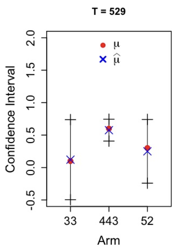Figure 1: The best arm is selected most of the time, also we noticed that its confidence interval is smaller than the other arms.

The uncertainty term $\sqrt{\frac{\gamma \log(t)}{2N_a(t-1)}}$, we can derive by leveraging Hoeffding-Chernoff bounds. We recall to these inequalities \eqref{eq:hoeffding} \eqref{eq:chernoff}. Given Hoeffding’s inequality for bounded random variables $X_i \in [0, 1]$ with $\mathbb{E}[X_i] = \mu$, $n$ independent sample, we can simplify the bound \eqref{eq:hoeffding} to:

\[\mathbb{P}\left(\left| \frac{1}{n} \sum_{i=1}^{n} X_i - \mu \right| \geq \epsilon\right) \leq 2 \exp\left(-2n\epsilon^2\right).\]

In context of UCB, $n$ we adjust for the number of pulls $N_a(t-1)$ of arm $a$ up to time $t-1$. Now we set probability of error $\delta$ and solve for $\epsilon$:

\[\begin{aligned} \delta & = 2 \exp\left(-2N_a(t-1)\epsilon^2\right) \\ \log\left(\frac{\delta}{2}\right) & = -2N_a(t-1)\epsilon^2 \\ \epsilon & = \sqrt{\frac{1}{2N_a(t-1)} \log\left(\frac{2}{\delta}\right)} \end{aligned}\]

Given dynamic adjustment for $\delta$, we can set $\delta = \frac{2}{t^\gamma}$, where $t$ is the time step and $\gamma$ is a parameter that controls the balance between exploration and exploitation. Plugging this in we have:

\[\begin{aligned} \epsilon & = \sqrt{\frac{1}{2N_a(t-1)} \log\left(\frac{2}{\frac{2}{t^\gamma}}\right)} \\ & = \sqrt{\frac{1}{2N_a(t-1)} \log(t^\gamma)} \\ & = \sqrt{\frac{1}{2N_a(t-1)} \gamma \log(t)} \\ & = \sqrt{\frac{\gamma \log(t)}{2N_a(t-1)}} \end{aligned}\]